Simple linear regression output interpretation

Question

I have run a simple linear regression of the natural log of 2 variables to determine if they correlate. My output is this:

R^2 = 0.0893

slope = 0.851

p < 0.001

I am confused. Looking at the $R^2$ value, I would say that the two variables are not correlated, since it is so close to $0$. However, the slope of the regression line is almost $1$ (despite looking as though it's almost horizontal in the plot), and the p-value indicates that the regression is highly significant.

Does this mean that the two variables are highly correlated? If so, what does the $R^2$ value indicate?

I should add that the Durbin-Watson statistic was tested in my software, and did not reject the null hypothesis (it equalled $1.357$). I thought that this tested for independence between the $2$ variables. In this case, I would expect the variables to be dependent, since they are $2$ measurements of an individual bird. I'm doing this regression as part of a published method to determine body condition of an individual, so I assumed that using a regression in this way made sense. However, given these outputs, I'm thinking that maybe for these birds, this method isn't suitable. Does this seem a reasonable conclusion?

Answer 1

The estimated value of the slope does not, by itself, tell you the strength of the relationship. The strength of the relationship depends on the size of the error variance, and the range of the predictor. Also, a significant $p$-value doesn't tell you necessarily that there is a strong relationship; the $p$-value is simply testing whether the slope is exactly 0. For a sufficiently large sample size, even small departures from that hypothesis (e.g. ones not of practical importance) will yield a significant $p$-value.

Of the three quantities you presented, $R^2$, the coefficient of determination, gives the greatest indication of the strength of the relationship. In your case, $R^{2} = .089$, means that $8.9\%$ of the variation in your response variable can be explained a linear relationship with the predictor. What constitutes a "large" $R^2$ is discipline dependent. For example, in social sciences $R^2 = .2$ might be "large" but in controlled environments like a factory setting, $R^2 > .9$ may be required to say there is a "strong" relationship. In most situations $.089$ is a very small $R^2$, so your conclusion that there is a weak linear relationship is probably reasonable.

Answer 2

The $R^{2}$ tells you how much variation of the dependent variable is explained by a model. However, one can interpret the $R^{2}$ as well as the correlation between the original values of the dependent variable and the fitted values. The exact interpretation and derivation of the coefficient of determination $R^{2}$ can be found here.

The proof that the coefficient of determination is the equivalent of the Squared Pearson Correlation Coefficient between the observed values $y_{i}$ and the fitted values $\hat{y}_{i}$ can be found here.

The $R^{2}$ or coefficient of determination indicates the strength of your model in explain the dependent variable. In your case, $R^{2}=0.089$. This that your model is able explain 8.9% of variation of you dependent variable. Or, the correlation coefficient between your $y_{i}$ and your fitted values $\hat{y}_{i}$ is 0.089. What constitutes a good $R^{2}$ is discipline dependent.

Finally, to the last part of your question. You cannot get the Durbin-Watson test to say something about the correlation between you dependent and independent variables. The Durbin-Watson test tests for serial correlation. It is conducted to examine whether your error terms are mutually correlated.

Answer 3

The $R^2$ value tells you how much variation in the data is explained by the fitted model.

The low $R^2$ value in your study suggests that your data is probably spread widely around the regression line, meaning that the regression model can only explain (very little) 8.9% of the variation in the data.

Have you checked to see whether a linear model is appropriate? Have a look at the distribution of your residuals, as you can use this to assess the fit of the model to your data. Ideally, your residuals should not show a relation with your $x$ values, and if it does, you may want to think of rescaling your variables in a suitable way, or fitting a more appropriate model.

Answer 4

For a linear regression, the fitted slope is going to be the correlation (which, when squared, gives the coefficient of determination, the $R^2$) times the empirical standard deviation of the regressand (the $y$) divided by the empirical standard deviation of the regressor (the $x$). Depending on the scaling of the $x$ and $y$, you can have a fit slope equal to one but an arbitrarily small $R^2$ value.

In short, the slope is not a good indicator of model 'fit' unless you are certain that the scales of the dependent and independent variables must be equal to each other.

Answer 5

@Macro had a great answer.

The estimated value of the slope does not, by itself, tell you the strength of the relationship. The strength of the relationship depends on the size of the error variance, and the range of the predictor. Also, a significant pp-value doesn't tell you necessarily that there is a strong relationship; the pp-value is simply testing whether the slope is exactly 0.

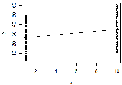
I just want to add a numerical example to show what is looks like to have a case OP described.

• Low $R^2$
• Significant on p-value

• Slope close to $1.0$

  set.seed(6)
  y=c(runif(100)*50,runif(100)*50+10)
  x=c(rep(1,100),rep(10,100))
  plot(x,y)
  
  fit=lm(y~x)
  summary(fit)
  abline(fit)
  
  
  > summary(lm(y~x))
  
  Call:
  lm(formula = y ~ x)
  
  Residuals:
     Min     1Q Median     3Q    Max 
  -24.68 -13.46  -0.87  14.21  25.14 
  
  Coefficients:
              Estimate Std. Error t value Pr(>|t|)    
  (Intercept)  25.6575     1.7107  14.998  < 2e-16 ***
  x             0.9164     0.2407   3.807 0.000188 ***
  ---
  Signif. codes:  0 ‘***’ 0.001 ‘**’ 0.01 ‘*’ 0.05 ‘.’ 0.1 ‘ ’ 1
  
  Residual standard error: 15.32 on 198 degrees of freedom
  Multiple R-squared:  0.0682,    Adjusted R-squared:  0.06349 
  F-statistic: 14.49 on 1 and 198 DF,  p-value: 0.0001877
  

Answer 6

I like the answers already given, but let me complement them with a different (and more tongue-in-cheek) approach.

Suppose we collect a bunch of observation from 1000 random people trying to find out if punches in the face are associated with headaches:

$$Headaches = \beta_0 + \beta_1 Punch\_in\_the\_face + \varepsilon $$

$\varepsilon$ contains all the omitted variables that produce headaches in the general population: stress, how contaminated your city is, lack of sleep, coffee consumption, etc.

For this regression, the $\beta_1$ might be very significant and very big, but the $R^2$ will be low. Why? For the vast majority of the population, headaches won't be explained much by punches in the face. In other words, most of the variation in the data (i.e. whether people have few or a lot of headaches) will be left unexplained if you only include punches in the face, but punches in the face are VERY important for headaches.

Graphically, this probably looks like a steep slope but with a very big variation around this slope.