An example of autocorrelation in residuals causing misinterpretation

Question

I'm looking for an example of time series data where a regression of y~x has autocorrelation in the residuals that leads to misinterpreting the model. This is for a class demonstration where I would ideally show them the results of an OLS model and the results of a GLS model with an appropriate correlation structure and explain the differences in the coefficients and their standard errors. Any examples out there that folks have used?

Answer 1

Chapter 5 in this textbook:

Heij, De Boer, Franses, Kloek and Van Dijk (2004) Econometric Methods with Applications in Business and Economics. Oxford University Press

uses two examples to illustrate how to test and interpret the presence of autocorrelation in the residuals from the classical regression model. Below I summarize the idea of these examples.

As you mention that it is for a class demonstration, I would recommend you the software gretl. It contains several data sets from textbooks in Econometrics as well as the necessary tools to reproduce most of the examples on those textbooks. You can check the data sets that are available here. If you have any of these textbooks you will probably find there an example that is suited for your purposes.

---

The first of the examples mentioned before uses economic time series data (interest and bond rates, available here). The authors explain that the presence of autocorrelation in the residuals of a static regression of changes in the bond rate on changes in Treasury Bill rates suggests that the model is not correctly specified. As it often happens with economic data, some of the dynamics is not captured by a static model. A possible reason is that adjustments to deviations from an equilibrium relationship among the variables may take more than one period. Upon this interpretation, a dynamic model with one lag of the dependent and explanatory variables is fitted and tested against the static model.

The second example uses cross-section data (income and consumption of food in 48 households of comparable size, available here). A model for expenditure as a linear function of total consumption and average household size is fitted. Then the authors show that Breusch and Godfrey test suggests the presence of autocorrelation. Similarly to the other example, this result is interpreted as a misspecification of the model. In the context of cross-section data adding lags of variables does not make much sense. The authors propose instead a non-linear relationship among the variables, which is fitted through non-linear least squares.

Answer 2

The following not only answers the OP's question about a data set that requires more than a simple OLS solution BUT also answers more general questions (unasked by the OP) regarding other possible deficiencies of OLS When applied to time series data. I use AUTOBOX here ( a piece of software I have helped develop) but one could use any software that can incorporate user-specified predictors while identifying an appropriatw arima structure and the need for any necessary unspecified dummy variables reflecting unspecified deterministic changes in the data. For a simpler problem set (less complicated solution required) just use the first 68 values.

TIME SERIES DATA

In http://www.autobox.com/stack/yaffe.xlsx we have 134 months of data ( Y first then X) . The OLS solution is here 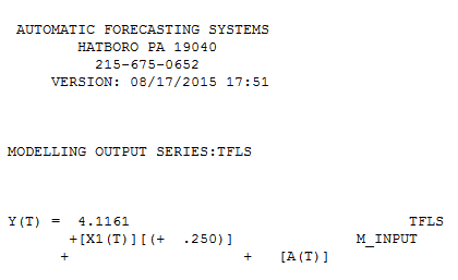with model statistics 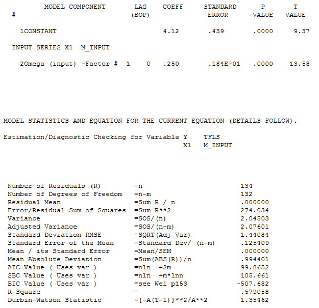. The acf of the residuals suggest model inadequacy 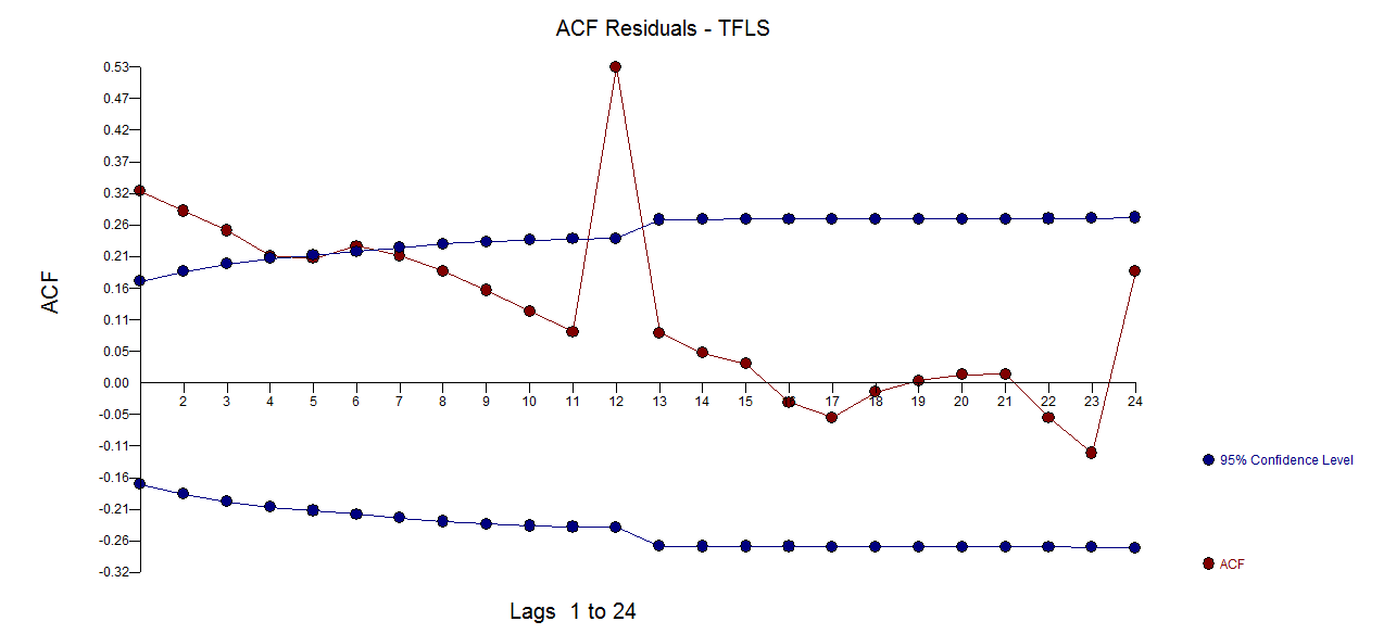. The actual/fit and forecast graph is here 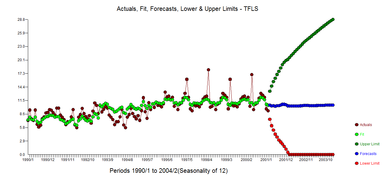suggesting clumps of non-zero residuals. The actual plot of these questionable residuals is here 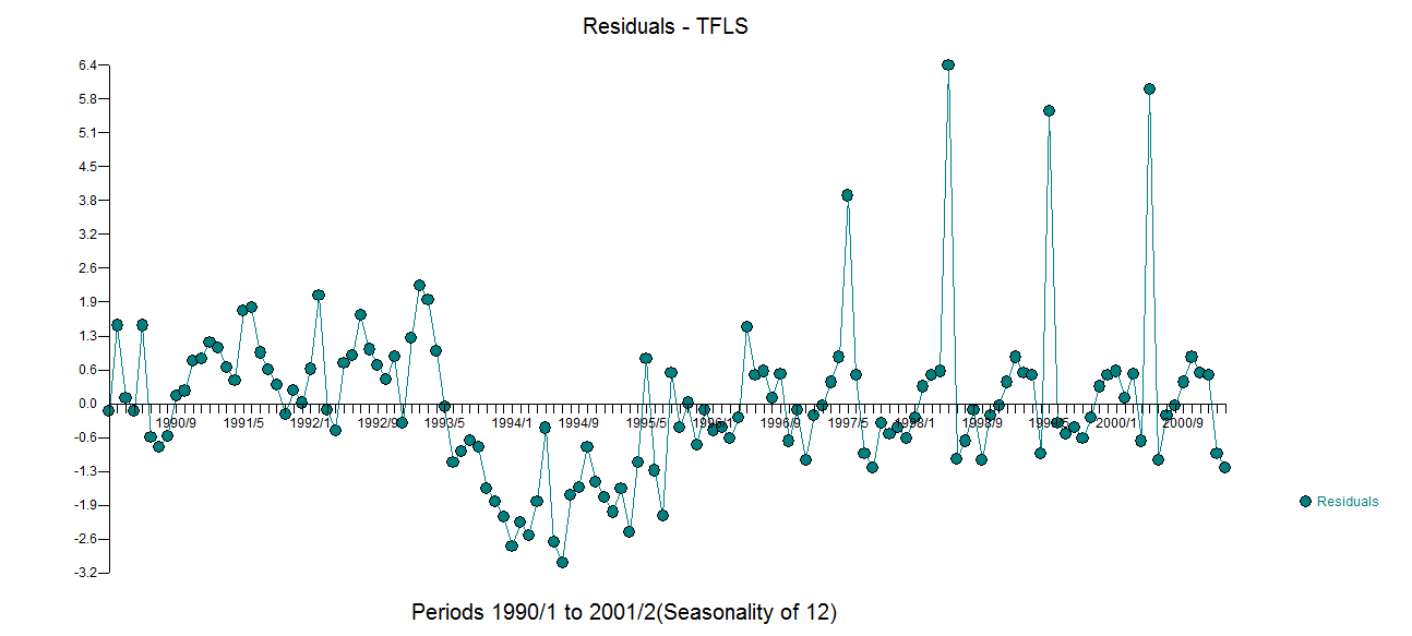A comprehensive approach GLS suggests not only suggests the existence/presence of auto-correlative structure but the impact of a level shift, seasonal pulse and some one-time only pulses in addition to a lag/delayed effect of the user-specified predictor variable X. Here is the GLS model 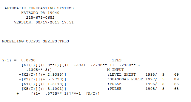and here 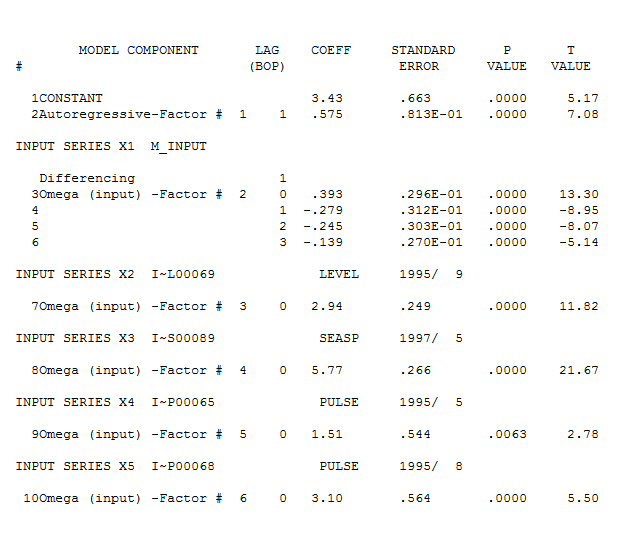with final model statistics here 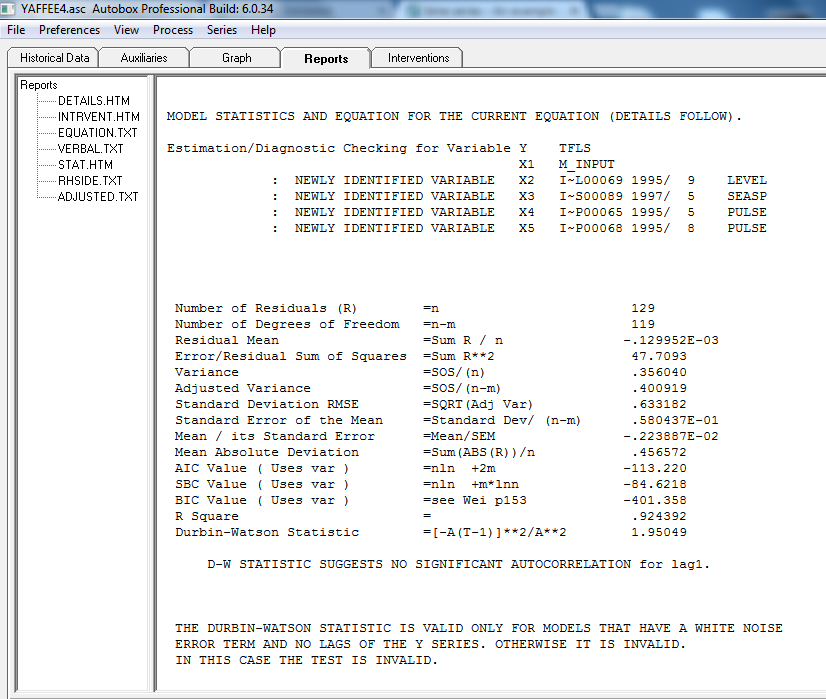. The plot of the acf of the residuals appears to suggest model sufficiency 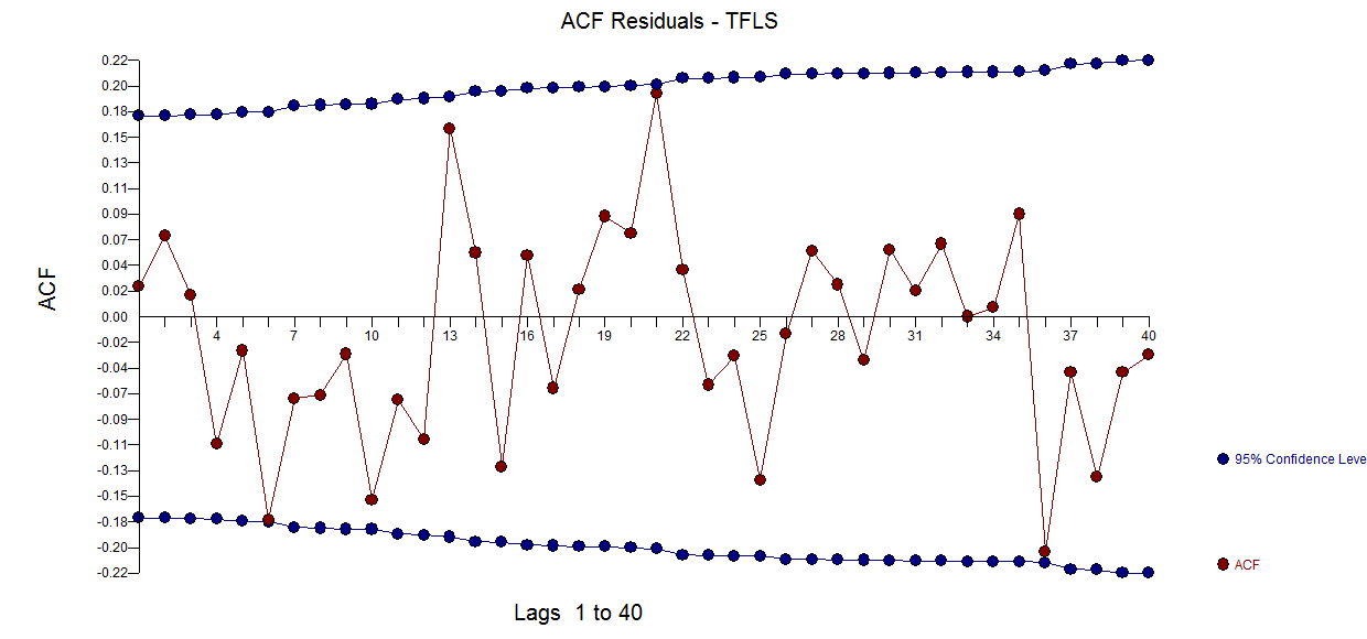with residual plot 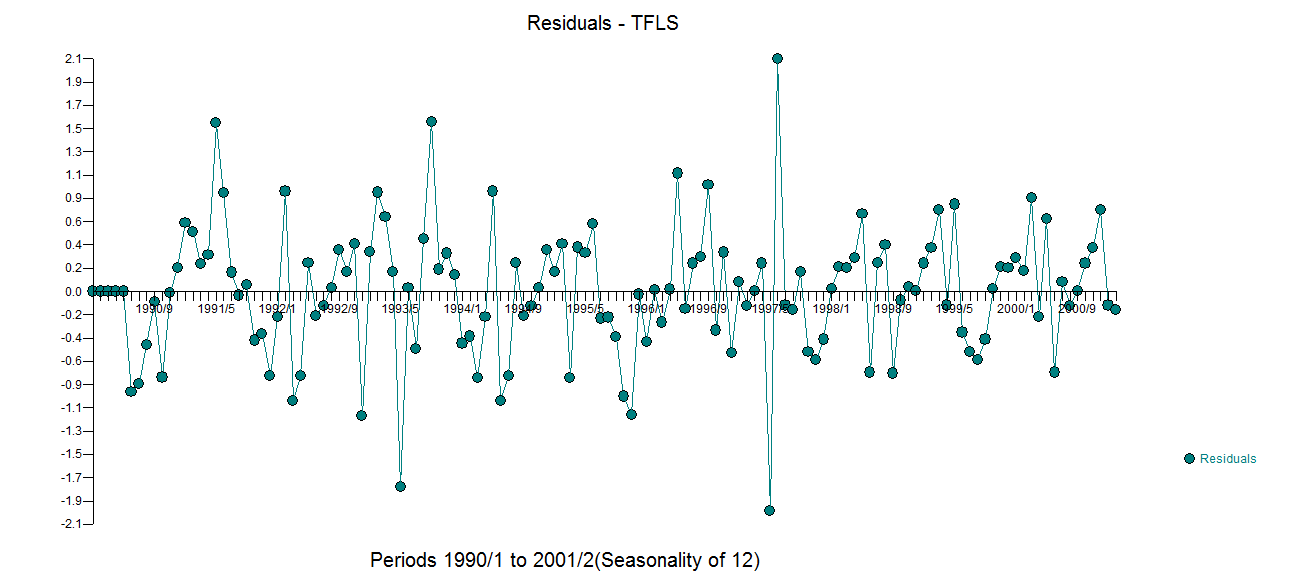and a respectable 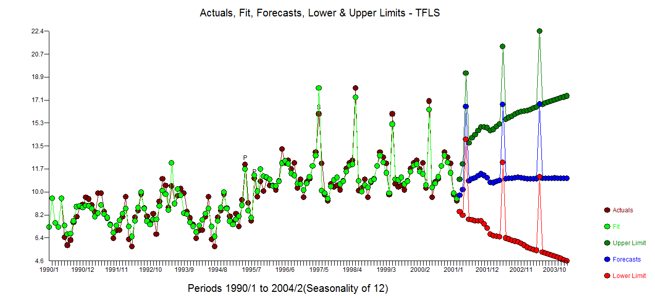looking actual . fit and forecast graph . Note that a GLS soultion not only deals with off-diagonal effects but possible variance change effects (not seen in this example) AND non-constancy in the expected error term (found in this example by the inclusion of a level shift and a seasonal pulse and a few one-time anomalies. Here is the plot of the acf for the errors from this model 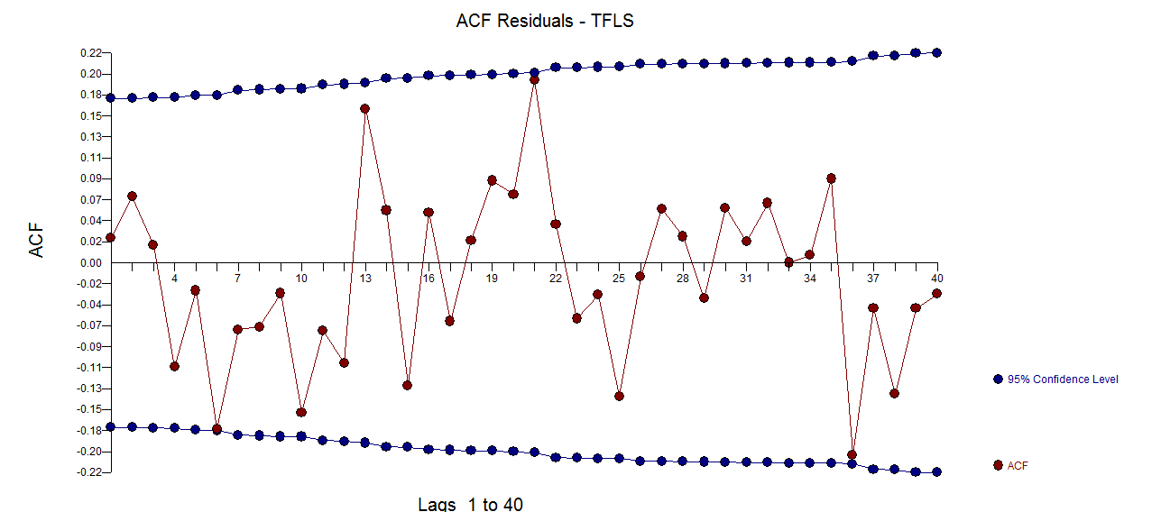suggsting sufficiency.