Estimate accuracy of an estimation on Poisson binomial distribution

Question

I manage a website that charges its customers using payment cards. Some transactions area approved, others are declined. I compute the approval rate of transactions for a interval (a calendar day) as the number of approved transactions (A) divided by the total number of transactions (T) processed during the specified time interval.

Example:

          | Approved | Declined | Total |       Approval Rate (R)
          |    (A)   |    (D)   |  (T)  |   (A/T) || A/(T+3) | (A+3)/(T+3)
----------+----------+----------+-------+---------++---------+-------------
yesterday |    50    |    29    |   79  |  0.6329 ||  0.6097 |   0.6463
today     |     7    |     4    |   11  |  0.6363 ||  0.5000 |   0.7142

The approval rates (R=A/T, the 4th column) are very close but it's obvious that the second one is not very reliable. Three more transactions make the today's rate change a lot (0.5000 .. 0.7142, the last two columns) but they have much smaller impact on yesterday's rate (because yesterday's rate is computed using a larger set of transactions).

What I need: based on the above facts I need a way (algorithm, formula) to compute or estimate the accuracy of the approval rate computed as above. A confidence level or something like this. Or a range where the approval rate is expected to be in the next hours of the day (with a certain probability, of course). Or a different way to estimate the approval rate and get a result that makes it clear that the 0.6329 of yesterday is more reliable than the 0.6363 of today.

Or something else, I don't know...

I have a very limited knowledge and understanding of statistics; I tried to express the facts as well as I could using plain English. After reading several articles on Wikipedia I found out that my problem is a Poisson binomial distribution (I hope I identified it correctly). I think the approval rate I compute is an estimation of the probability of the distribution but I don't have any idea what parameter models the information I need and how to compute it.

Answer 1

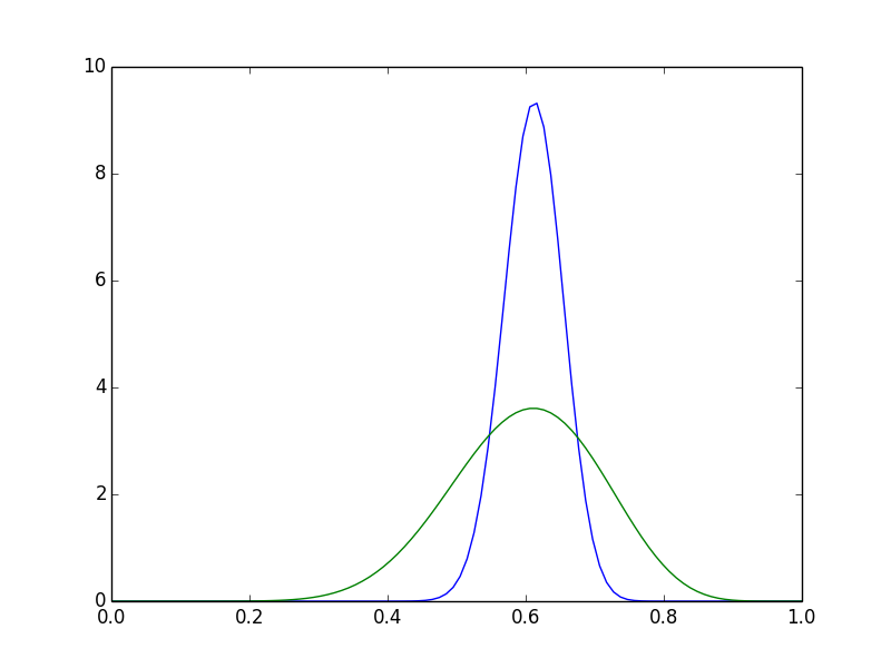
If your sole need is to express your relative uncertainty in the probability of a declined transaction each day, it would seem you could fit a simple beta-binomial model. In this model, each of $n$ total transactions has the same probability $p$ of success, and there are $k$ total successes.

If you took the cookie-cutter Bayesian approach and assumed this value was equally likely to be any value between $0$ and $1$ at the start of each day, then the uncertain estimate you're looking for could be expressed as a $Beta(n + 1, k + 1)$ distribution. You could then use summary statistics, say the 95% highest-density interval, to express this uncertainty.

For your data, these distributions would produce plots like this (Python code to produce them below):

from matplotlib import pylab as plt
from scipy.stats import beta
x = np.linspace(0,1,100)
y1 = beta.pdf(x, 80, 51)
y2 = beta.pdf(x, 12, 8)
plt.plot(x, y1)
plt.plot(x, y2)

Answer 2

1. If you can assume that, on the same day, all cards have equal probability of approval

You try to estimate an unknown appoval rate for each day, let us call this unknown rate $p$. On one day you observe a number of events $N$ (79 yesterday and 11 today). If you assume that all events are independent and that at each individual event the unknown rate (a probability) is the same then you have a Binomial random variable. For a Binomial random variable the expected value is $Np$ and the variance is $Np(1-p)$. So $X \sim Bin(N;p)$ X is the number of approvals you observe in a day and $\mu_X=Np,\sigma_X^2=Np(1-p)$.

The $p$ is unknown but can be estimates as the number of approvals divided by the total number of events in a day, so $\hat{p}=\frac{A}{T}$, which is what you compute.

So what you compute is $\frac{X}{N}$ where $\mu_X=Np,\sigma_X^2=Np(1-p)$. But if $\mu_x=N.p$ then the mean of $\frac{X}{N}$ is the mean of X divided by N, so $\mu_{(\frac{X}{N})}=\frac{\mu_X}{N}=\frac{Np}{N}=p$ therefore you have an unbiased estimator of the unknown $p$.

The variance of $\frac{X}{N}$ is the variance of $X$ divided by $N^2$, so it is $\frac{Np(1-p)}{N^2}=\frac{p(1-p)}{N}$. The square root of the variance is the standard deviation. This standard deviation of your estimator is a measure of imprecision: the larger it is, the more imprecise your estimate.

So in your case, for day 1, $\hat{p}=\frac{50}{79}=0.63$ and the standard deviation on it is $\sqrt{\frac{p(1-p)}{N}}$ which can be approximated by replacinig $p$ with $\hat{p}$. So the standard deviation is $\sqrt{\frac{0.63\times0.37}{79}}=0.054$, the larger this standard deviation, the more imprecise your estimate is.

On the second day you find $\hat{p}=0.64$ with a 'imprecision' of $\sqrt{\frac{0.64\times0.36}{11}}=0.14$, so a larger standard deviation and thus less precise.

2. If you can assume that, on the same day, all cards have equal probability of approval, AND this probability is the same every day

If you can reasonably assume that on all days this rate will be the same, then you can increase the precision of your estimate by ''pooling''; indeed, on day 1 you have a binomial with success probability p and size 79, on day two these are respectively p and 11, and the sum of two independent binomials is again binomial, so in that case you have Bin(p;90) and you observe 57 approvals, so $\hat{p}=\frac{57}{90}=0.63$ and the 'imprecision' is $\sqrt{ \frac{0.63 \times 0.37}{90}}=0.050$

3. If you can NOT assume that, on the same day, all cards have equal probability of approval

If you can not assume that, within each day, all events have the same $p$, then you have sums of Bernouilli variables with different succes probability and your random variable is no longer Binomial but so-called Poisson-Binomial. The idea is similar, the estimate for the rate is the same, but your variance of Poisson-Binomial has a correction term ( -N times the variance of the p's, this variance of the p's must be estimated from your data, as you subtract this amount, the variance will be smaller: $Np(1-p) - N \times Var(p)$ in stead of $Np(1-p)$ for the Binomial).

So the only difference is the formula for the variance, the rest is similar, but I don't see how to estimate Var(p) with your data.

4. Responses to the comment(s)

@axiac: If you say that "no day is like any other day" then it can still be that the probabilities $p$ above are different between the days BUT within one day an individual transaction has the same probability of approval $p_{day}$. If that is a reasonable assumption then you are in case 1.

If the probability of approval is realy different from transaction to transaction, even for transactions on the same day, then the only difference between case 3 and case 1 is the formula for the variance: your estimate $\hat{p}$ is then an estimator of the average of all (different) $p_{transaction}$ and the variance is computed as $\frac{\hat{p}(1-\hat{p}) - Var(p_{transaction})}{N}$

So if the variance of the probability of approval over all transactions is not too large, then you can 'assume away' the second term and you are back in case 1. If You think that there is considerable $Var(p_{transaction})$ (i.e. large compared to $\hat{p}(1-\hat{p})$) then you have to find an estimate of the variance of the p's. The only one I can think of is that you compute the proportions on several days, and then use the variance of these proportions as your estimate of $Var(p_{transction})$.