Bayesian analysis of a probability of success

Question

Let $S \sim \text{Bin}(N, \pi)$ denote a number of successes. Using the non-informative $\text{Beta}(0.5, 0.5)$ prior, the posterior distribution of the probability of success is $$ \text{Beta}(0.5 + S, \, 0.5 + N - S) $$

Say that the interest is in the posterior probability that $\pi > 0.60$, i.e.

$$ \text{Pr}\big(\text{Beta}(0.5 + S, \, 0.5 + N - S) > 0.60\Big) $$

The R function f() below assumes that the true $\pi$ equals $0.8$ and computes the proportion of times, over 10000 simulations, that this posterior probability is $> 0.95$.

f <- function(N, pi=0.8)
{
  S <- rbinom(n=10000, size=N, prob=pi)
  proba <- 1 - pbeta(0.60, 0.5 + S, 0.5 + N - S)
  mean(proba > 0.95)
}

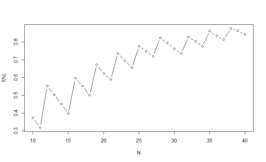
I would expect $f$ to be an increasing function of $N$ (after all, the posterior distribution becomes increasingly concentrated around $0.80 > 0.60$ as $N$ increases).

However,

Do you have an explanation for the behaviour?

Answer 1

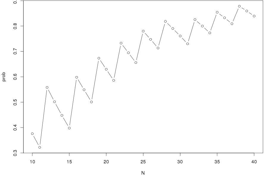
It occurs because $S$ is discrete.

For every value $N$, there is a certain value of $S$, call it $S_N$, such that the posterior probability of $\pi>0.6$ is greater than 0.95. We can find $S_N$ using this R function:

find_cutoff = function(N) {
  s = 0:N
  min(s[which(1-pbeta(.6, .5+s, .5+N-s) > .95)])
}

Now that we have the cutoff, we need to find the probability that $S\ge S_N|N$ which is just evaluating one minus the cdf of a binomial distribution.

library(plyr)
d = ddply(data.frame(N=10:40), .(N), function(x){
  cutoff = find_cutoff(x$N)
  data.frame(cutoff = cutoff,
         prob = 1-pbinom(cutoff-1, x$N, .8))
})
plot(prob~N,d, type='b')