Time series for count data, with counts < 20

Question

I recently started working for a tuberculosis clinic. We meet periodically to discuss the number of TB cases we're currently treating, the number of tests administered, etc. I'd like to start modeling these counts so that we're not just guessing whether something is unusual or not. Unfortunately, I've had very little training in time series, and most of my exposure has been to models for very continuous data (stock prices) or very large numbers of counts (influenza). But we deal with 0-18 cases per month (mean 6.68, median 7, var 12.3), which are distributed like this:

[image lost to the mists of time]

[image eaten by a grue]

I've found a few articles that address models like this, but I'd greatly appreciate hearing suggestions from you - both for approaches and for R packages that I could use to implement those approaches.

EDIT: mbq's answer has forced me to think more carefully about what I'm asking here; I got too hung-up on the monthly counts and lost the actual focus of the question. What I'd like to know is: does the (fairly visible) decline from, say, 2008 onward reflect a downward trend in the overall number of cases? It looks to me like the number of cases monthly from 2001-2007 reflects a stable process; maybe some seasonality, but overall stable. From 2008 through the present, it looks like that process is changing: the overall number of cases is declining, even though the monthly counts might wobble up and down due to randomness and seasonality. How can I test if there's a real change in the process? And if I can identify a decline, how could I use that trend and whatever seasonality there might be to estimate the number of cases we might see in the upcoming months?

Answer 1

To assess the historical trend, I'd use a gam with trend and seasonal components. For example

require(mgcv)
require(forecast)
x <- ts(rpois(100,1+sin(seq(0,3*pi,l=100))),f=12)
tt <- 1:100
season <- seasonaldummy(x)
fit <- gam(x ~ s(tt,k=5) + season, family="poisson")
plot(fit)

Then summary(fit) will give you a test of significance of the change in trend and the plot will give you some confidence intervals. The assumptions here are that the observations are independent and the conditional distribution is Poisson. Because the mean is allowed to change smoothly over time, these are not particularly strong assumptions.

To forecast is more difficult as you need to project the trend into the future. If you are willing to accept a linear extrapolation of the trend at the end of the data (which is certainly dodgy but probably ok for a few months), then use

fcast <- predict(fit,se.fit=TRUE,
               newdata=list(tt=101:112,season=seasonaldummyf(x,h=12)))

To see the forecasts on the same graph:

plot(x,xlim=c(0,10.5))
lines(ts(exp(fcast$fit),f=12,s=112/12),col=2)
lines(ts(exp(fcast$fit-2*fcast$se),f=12,s=112/12),col=2,lty=2)
lines(ts(exp(fcast$fit+2*fcast$se),f=12,s=112/12),col=2,lty=2)

You can spot the unusual months by looking for outliers in the (deviance) residuals of the fit.

Answer 2

You might want to have a look at strucchange:

Testing, monitoring and dating structural changes in (linear) regression models. strucchange features tests/methods from the generalized fluctuation test framework as well as from the F test (Chow test) framework. This includes methods to fit, plot and test fluctuation processes (e.g., CUSUM, MOSUM, recursive/moving estimates) and F statistics, respectively. It is possible to monitor incoming data online using fluctuation processes. Finally, the breakpoints in regression models with structural changes can be estimated together with confidence intervals. Emphasis is always given to methods for visualizing the data."

PS. Nice graphics ;)

Answer 3

Does it really need some advanced model? Based on what I know about TB, in case there is no epidemy the infections are stochastic acts and so the count form month N shouldn't be correlated with count from month N-1. (You can check this assumption with autocorrelation). If so, analyzing just the distribution of monthly counts may be sufficient to decide if some count is significantly higher than normal.
On the other hand you can look for correlations with some other variables, like season, travel traffic, or anything that you can imagine that may be correlated. If you would found something like this, it could be then used for some data normalization.

Answer 4

You may try to model your data using a Dynamic Generalized Linear Model (DGLM). In R, you can fit this kind of models using packages sspir and KFAS. In a sense, this is similar to the gam approach suggested by Rob, except that instead of assuming that the log mean of the Poisson observations be a smooth function of time, it assumes that it follows a stochastic dynamics.

Answer 5

Often, disease data like this is performed with a generalized linear model, as its not necessarily a great application of time series analysis - the months often aren't all that correlated with each other.

If I were given this data, here's what I would do (and indeed, have done with data similar to it):

Create a "time" variable that's more accurately described as "Months since 1/1/2000" if I'm eyeballing your data correctly. Then I'd run a general linear model in R using the Poisson distribution (or Negative Binomial) and a log link with roughly the following form:

log(Counts) = b0 + b1*t + b2*(t^2) + b3*cos(2pi*w*t) + b4*sin(2pi*w*t)

Where t is the time described above, and w is 1/365 for a yearly disease like flu. Generally its 1/n, where n is the length of your disease's cycle. I don't know offhand what it is for TB.

The two time trends will show you - outside normal seasonal variation - if you have meaningful variation over time.

Answer 6

You might consider applying a Tukey Control chart to the data.

Answer 7

I'm going to leave the main question alone, because I think I will get it wrong (although I too analyse data for a healthcare provider, and to be honest, if I had these data, I would just analyse them using standard techniques and hope for the best, they look pretty okay to me).

As for R packages, I have found the TSA library and it's accompanying book very useful indeed. The armasubsets command, particularly, I think is a great time saver.

Answer 8

Escape from traditional enumerative statistics as Deming would suggest and venture into traditional analytical statistics - in this case, control charts. See any books by Donald Wheeler PhD, particularly his "Advanced Topics in SPC" for more info.

Answer 9

In response to your direct question "How can I test if there's a real change in the process? And if I can identify a decline, how could I use that trend and whatever seasonality there might be to estimate the number of cases we might see in the upcoming months?" Develop a Transfer Function Model ( ARMAX ) that readily explains period-to-period dependency including and seasonal ARIMA structure. Incorporate any Identifiable Level Shifts , Seasonal Pulses, Local Time Trends and PUlses that may have been suggested by empirical/analystical methods like Intervention Detection. IF THIS ROBUST MODEL INCLUDES A FACTOR/SERIES matching up with "declines" Then your prayers have been answerered. In the alternative simply add an hypothesized structure e.g. to test a time trend change at point T1 construct two dummies X1 = 1,1,2,3,,,,,,T and X2 = 0,0,0,0,0,0,0,1,2,3,4,5,.... WHERE THE ZEROES END AT PERIOD T1-1 . The test of the hypothesis of a significant trend change at time period T1 will be assessed using the "t value" for X2 .

Edited 9/22/11

Often, disease data like this has monthly effects since weather/temperature is often an unspecified causal . In the omission of the true caudsal series ARIMA models use memory or seasonal dummies as a surrogate. Additionally series like this can have level shifts and/or local time trends reflecting structural change over time. Exploiting the autoregressive structure in the data rather than imposing various artifacts like time and time square and time cubic etc. have been found to be quite useful and less presumptive and ad hoc. Care should also be taken to identify "unusual values" as they can often be useful in suggestng additional cause variables and at a minimum lead to robust estimates of the other model parameters. Finally we have found that the variability/paramaters may vary over times thus these model refinements may be in order.

Answer 10

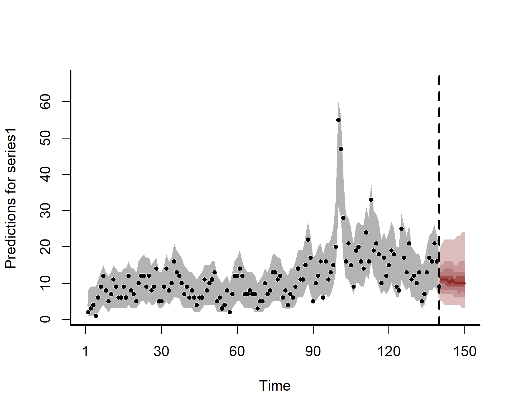
For modeling integer-valued time series (or any non-Gaussian time series), I would opt for a State-Space model that allows the latent dynamic process to evolve independently of the observations. This is very useful when dealing with observations that have restrictions, such as non-negative integers, proportional values, or observations that require offsets, because we can let the latent dynamic process be real-valued and use the convenience of link functions (like we do in Generalized Linear Models) to translate to the observation scale. My package {mvgam} was designed specifically for this kind of situation because I frequently have to analyse and forecast multivariate sets of count-valued time series with missing values, many zeros and overdispersion, and none of the more commonly used methods (such as the INAR) are capable of dealing with all of these features. I also wanted the ability to include nonlinear smooth functions of covariates (using Generalized Additive Models) in both the latent process model and in the observation model, because again many real-world time series have observation error that needs to be captured.

The general formula for Dynamic Generalized Additive Models is:

$$for~i~in~1:N_{series}~...$$ $$for~t~in~1:N_{timepoints}~...$$ $$g^{-1}(\tilde{\boldsymbol{y}}_{i,t})=\alpha_{i}+\sum\limits_{j=1}^Js_{i,j,t}\boldsymbol{x}_{j,t}+Zz_{i,t}\,,$$

Here $\alpha$ are the unknown intercepts, the $\boldsymbol{s}$'s are unknown smooth functions of covariates ($\boldsymbol{x}$'s), which can potentially vary among the response series, and $z$ are dynamic latent processes. Each smooth function $s_j$ is composed of basis expansions whose coefficients, which must be estimated, control the functional relationship between $\boldsymbol{x}_{j}$ and $g^{-1}(\tilde{\boldsymbol{y}})$. The size of the basis expansion limits the smooth’s potential complexity. A larger set of basis functions allows greater flexibility. In {mvgam} you can use any basis that is available in {mgcv}, including specialized cyclic bases that are very useful for detecting seasonality. Note that we can also include linear predictors for the $z$, which is often useful to do, and we can impose a wide variety of temporal dynamic structures (such as Random Walk, AR processes, Continuous Time AR processes, or even Vector Autoregressions). The $Z$ matrix affords even more flexibility by letting some series share the same latent process model (i.e. perhaps two observation series are tracking the same hidden process, but with different observation errors). For more information on GAMs and how they can smooth through data, see this blogpost on how to interpret nonlinear effects from Generalized Additive Models.

To see how this can work for integer-valued time series, you can read through this short worked example.