How to analyze $ 2\times n$ contingency table?

Question

I have a $2\times n$ contingency table. I want to assess whether the rows are independent from the columns or not. If not, I want to know which columns are not independent and which are.

What tests are available to analyze these kind of data?

Addendum: In particular, what to do when some of the entries in the table are very small or zero?

Answer 1

I've looked into it using [R], and I am a bit surprised to see no packaged formula readily accessible for a test that is ubiquitous in the medical sciences. So it takes some minimal tweaking. First off, the link in my comment to the OP is excellent, providing a makeshift formula; however, the following is an example using well-known formulas in [R]:

1. LARGER SAMPLES (> 5 expected counts in each cell):

I'll work with a toy example that I made up for a different post in CV, summarized into a contingency table comparing how many patients suffered heartburn after being treated with two kinds of antacids. For your question, I have extended the data to a third antacid as follows:

Antacid <- matrix(c(64, 178 - 64, 92, 190 - 92, 52, 188 - 52), nrow = 2)
dimnames(Antacid) = list(Symptoms = c("Heartburn", "Normal"),
                        Medication = c("Drug A", "Drug B", "Drug C"))
Antacid

               Medication
Symptoms       Drug A   Drug B   Drug C
  Heartburn     64       92       52
  Normal       114       98      136

First off, we can run an omnibus test (Pearson's $\chi^2$ "goodness-of-fit") on the data by simply calling prop.test, but there is just one minor problem: our data is in the form of a $2$ x $3$ matrix. Yet, the essential input into the function is a a two-dimensional table (or matrix) with 2 columns, giving the counts of successes and failures, i.e. an $n$ x $2$ matrix. Luckily the fix is easy: do a transpose of the matrix as follows:

t(Antacid)
          Symptoms
Medication    Heartburn    Normal
    Drug A        64        114
    Drug B        92         98
    Drug C        52        136

Now we are ready:

  prop.test(t(Antacid))
    3-sample test for equality of proportions without continuity correction

data:  t(Antacid)
X-squared = 17.6325, df = 2, p-value = 0.0001483
alternative hypothesis: two.sided
sample estimates:
   prop 1    prop 2    prop 3 
0.3595506 0.4842105 0.2765957 

So we know that we are not dealing with drugs of equal efficiency to treat heartburn, but we want to know more specifically what the pairwise comparisons have to say. Again, we have to stick with our transposed matrix t():

pairwise.prop.test(t(Antacid), p.adjust.method ="bonferroni")

Notice that to keep the probability of a type I error under check, I selected the Bonferroni method to adjust the p-values. The result is:

    Pairwise comparisons using Pairwise comparison of proportions 

data:  t(Antacid) 

       Drug A  Drug B 
Drug B 0.06221 -      
Drug C 0.33388 0.00015

P value adjustment method: bonferroni 

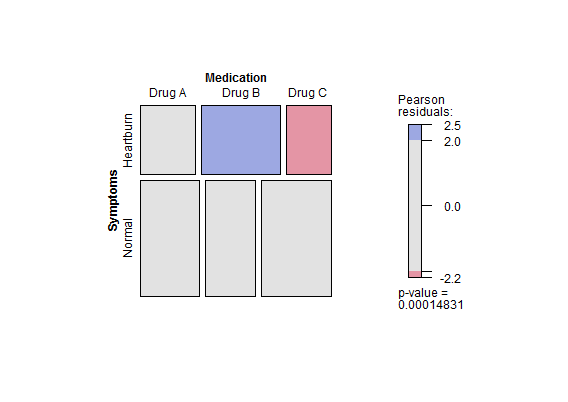
Interestingly, we can get this info all at once graphically simply with the following commands:

library(vcd)
mosaic(Antacid, shade=TRUE, legend=TRUE)

There you have it: when you look at the heartburn row, the square in pink, corresponding to Drug C is much smaller than Drug B (in blue), and the significance of the residuals (i.e. differences between expected and observed values for each entry, squared) are plotted to the right in terms of color hue: the darker the color (blue or pink) the larger the residuals. The residuals (distance from the expected value) can be exactly calculated to fully understand the plot by first summoning the table with marginal counts:

Antacid <- rbind(Antacid, margin.table(Antacid,2))
Antacid <- cbind(Antacid, margin.table(Antacid,1))
dimnames(Antacid) = list(Symptoms = c("Heartburn", "Normal","Totals"),
               Medication = c("Drug A", "Drug B", "Drug C", "Totals"))

               Medication
Symptoms    Drug A Drug B Drug C Totals
  Heartburn     64     92     52    208
  Normal       114     98    136    348
  Totals       178    190    188    556

Now we can see that the departure for Drug C number of heartburn sufferers from the number expected is in the negative territory:

Exp_burn <- Antacid[1,4] * Antacid[3,3] / Antacid[3,4]
(Antacid[1,3] - Exp_burn)/Exp_burn
[1] -0.2606383

Whereas for Drug B is a excess of sufferers to those predicted:

Exp_burn <- Antacid[1,4] * Antacid[3,2] / Antacid[3,4]
(Antacid[1,2]-Exp_burn)/Exp_burn
[1] 0.294332

And these results explain the color coding in terms of the hue of pink and blue.

The column to the right also includes the exact same p-value we just got for the pairwise $\chi^2$ of Drug B versus Drug C with Bonferroni adjustment.

2. SMALLER SAMPLES:

We use the Fisher exact test, which is based on the hypergeometric distribution, and it is probably most adequate when the expected values in any of the cells of a contingency table are below 5 - 10. Although originally conceived for $2$ x $2$ contingency tables, only the quickly mounting number of permutation tables in the extension of the Fisher test to $m$ x $n$ tables (so-called Freeman Halton test) gets in the way of its direct applications beyond the more rudimentary contingency table. This is discussed in CV, and elaborated further in this Wolfram post. The original article on the Freeman-Halton test can be found in Biometrika (1951) 38 (1-2): 141-149. doi: 10.1093/biomet/38.1-2.141.

Let's throw out subjects from our Antacid table, and reduce it in size so that the counts are low in each cell:

Antacid <- matrix(c(7, 11 - 7, 1, 15 - 4, 6, 9-6), nrow = 2)
dimnames(Antacid) = list(Symptoms = c("Heartburn", "Normal"),
                    Medication = c("Drug A", "Drug B", "Drug C"))

               Medication
Symptoms       Drug A  Drug B  Drug C
  Heartburn      7      1      6
  Normal         4     11      3

addmargins(Antacid) # Thanks for the tip @gung

               Medication
Symptoms       Drug A   Drug B   Drug C    Sum
  Heartburn      7         1      6        14
  Normal         4        11      3        18
  Sum           11        12      9        32

Clearly we would opt to take Drug B if given a choice. Let's look at the numbers, first globally:

fisher.test(Antacid)

        Fisher's Exact Test for Count Data

data:  Antacid
p-value = 0.008444
alternative hypothesis: two.sided

At this point we would reject the idea of these three drugs being equal.

Notice that as the table gets bigger computational issues may arise, explaining the command:

fisher.test(Antacid, simulate.p.value=TRUE)

Fisher's Exact Test for Count Data with simulated p-value (based on 2000 replicates)
    data:  Antacid 
    p-value = 0.009495 
    alternative hypothesis: two.sided

In this case the p-value is calculated through a Monte Carlo simulation.

Now for pairwise comparisons we can proceed as follows (notice how we need to transpose the matrix as explained above):

library(fmsb)
pairwise.fisher.test(t(Antacid), p.adjust.method = "bonferroni")

Pairwise comparisons using Pairwise comparison of proportions (Fisher) 

data:  t(Antacid) 

       Drug A Drug B
Drug B 0.028  -     
Drug C 1.000  0.047 

P value adjustment method: bonferroni 

So it is reasonable to conclude (assuming a risk $\alpha$ of 5%) that Drug B is different from both Drug A and Drug C.