I wish to run an ANOVA on 13 groups: each group has a different sample size. Also, my groups are not normal and it barely passed Levene's test at $p=.052$. I have tried transformations by square rooting and ln, but that only makes it worse. I tried to run a KWH test, but my data does not meet the variance test. Is there anything else I can do?
-
1$\begingroup$ What arew your sample sizes (in each group)? Can you post the data? Did you try box-cox transform? Can you spell out what is KWH test? $\endgroup$– kjetil b halvorsen ♦Commented Dec 2, 2015 at 15:05
-
$\begingroup$ My sample sizes range from 21 to 70, so I have a decent amount of sample data. I am not familiar with box-cox and KWH is kruskal wallis H test $\endgroup$– A. RomainCommented Dec 2, 2015 at 16:14
-
$\begingroup$ Can you post (as an edit to original post) a parallell boxplot of the 13 groups? That might be useful. You could use a version of one-way anova not assuming constant variance (like oneway.test in R), and you could combine that with bootstrapping. $\endgroup$– kjetil b halvorsen ♦Commented Dec 2, 2015 at 16:27
-
$\begingroup$ I posted a link to the google docs of my values and groups. And I didn't want to use one way ANOVA since the data is not normal. I know ANOVA is robust, but with violating equal variances I did not wish to try it $\endgroup$– A. RomainCommented Dec 2, 2015 at 16:30
-
3$\begingroup$ As commented variously by kjetil and @gung, these data seem puzzling, as they are in some senses implausibly well behaved for counts. Is there some generating process that you are not telling us about? As a very wild guess, are they the number of organisms out of some total with a particular property? $\endgroup$– Nick CoxCommented Dec 3, 2015 at 20:14
3 Answers
The data, as indicated by the variable names in the linked-to spreadsheet, pertains to number of organisms in 13 groups, so are some kind of count data. We could do better here if we knew some more about the data! But I do not agree with the answer by @gung that we should use some count data model, like Poisson regression. I will show graphically why I say that.
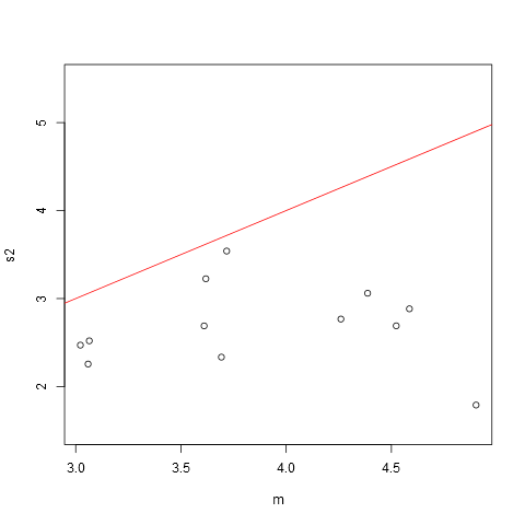
The Poisson distribution have variance equal to the mean, so a simple first analysis is to plot (empirical) variances against means. After reading the data into a data.frame (in R) I did:
> summary(dat)
     Number          Group
 Min.   :1.000   13     : 90
 1st Qu.:3.000   1      : 76
 Median :4.000   4      : 70
 Mean   :3.826   3      : 65
 3rd Qu.:5.000   6      : 62
 Max.   :8.000   12     : 62
                 (Other):299

>  s2<- with(dat, tapply(Number, Group, FUN=var))
>  m <- with(dat, tapply(Number, Group, FUN=mean))
> plot(m, s2, ylim=c(1.5, 5.5))
> abline(0, 1, col="red")
The red line shows variance equal to the mean. We see that all the points are below this line, and there is not much evidence that the variance increases with the mean either. So this is not Poisson data. Also, while the variances vary, they do not vary too much (all are within a factor of two), so the usual equal-variance Anova $F$ test can probably be used, as it is reasonably robust against small variations in the variance. The classic book by Miller: "Beyond Anova" gives a factor of four as acceptable. So let us try Anova in R, with and without that assumption:
> oneway.test(Number ~ Group, data=dat, var.equal=FALSE)

        One-way analysis of means (not assuming equal variances)

data:  Number and Group
F = 10.265, num df = 11.00, denom df = 265.99, p-value = 1.29e-15

> oneway.test(Number ~ Group, data=dat, var.equal=TRUE)

        One-way analysis of means

data:  Number and Group
F = 9.4014, num df = 11, denom df = 712, p-value = 6.497e-16
Both give basically the same conclusion here: the null hypothesis of equality of means is rejected. Note that the $F$ ratios are very similar.
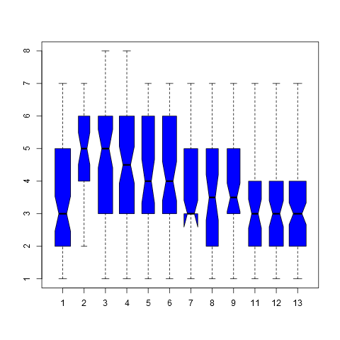
Let us also show a graphical analysis, a boxplot with "notches" showing confidence intervals for the median:
    > boxplot(Number ~ Group, data=dat, notch=TRUE, col="blue",
              varwidth=TRUE)
    Warning message:
    In bxp(list(stats = c(1, 2, 3, 5, 7, 2, 4, 5, 6, 7, 1, 3, 5, 6,  :
      some notches went outside hinges ('box'): maybe set notch=FALSE
We see that some of the confidence intervals do not overlap at all, again consistent with the Anova results. I would not be overly concerned with problems with the assumptions underlying Anova with this data, so the conclusion is quite robust. If wanted, it could be further analyzed with the bootstrap, but I will leave that to others. If further analysis is wanted, we would need more information about the data.
-
$\begingroup$ Thanks for all of your help and helping me analyze it better. So I can assume that the data differ among group. Now what post hoc test could I use? Scheffes? $\endgroup$ Commented Dec 3, 2015 at 15:14
-
1$\begingroup$ I did explicitly mention that the data were underdispersed relative to the Poisson, & I backed up the analysis with a chi-squared test that does not rely on those assumptions. $\endgroup$ Commented Dec 3, 2015 at 16:04
-
2$\begingroup$ gung Yes. What would be interesting here is understanding more about how this data was obtained, underdispersion is a quite special phenomenon, which often arises from some kind of negative correlations. The data are simply to regular to be Poisson! $\endgroup$ Commented Dec 3, 2015 at 16:14
-
1$\begingroup$ I'm sorry gung, I did not read your comments until after kjetil's. Thank you both for all of your help $\endgroup$ Commented Dec 3, 2015 at 17:09
-
1$\begingroup$ @kjetilbhalvorsen, they are too regular. It is rather suspicious. I'm afraid I know little about underdispersion. I am a bit leery of using an ANOVA here, but I haven't simulated these things, so I'm not sure how the different assumption violations trade off. $\endgroup$ Commented Dec 3, 2015 at 18:59
I notice that your response is called "Number of Organisms", and that all the values are non-negative integers. I suspect these are count data. They should not be treated as normally distributed and analyzed with a traditional ANOVA. Instead, a count GLM is appropriate. We can try Poisson regression:
anova(glm(N.Organisms~as.factor(Group), data=d, family=poisson), test="LRT")
# Analysis of Deviance Table
# Model: poisson, link: log
# Response: N.Organisms
# Terms added sequentially (first to last)
#
#                  Df Deviance Resid. Df Resid. Dev  Pr(>Chi)
# NULL                               723     619.31
# as.factor(Group) 12   78.907       711     540.41 6.669e-12 ***
# ---
# Signif. codes:  0 ‘***’ 0.001 ‘**’ 0.01 ‘*’ 0.05 ‘.’ 0.1 ‘ ’ 1

aggregate(N.Organisms~Group, data=d,
          FUN=function(x){  c(mean=mean(x),variance=var(x)) })
# Group N.Organisms.mean N.Organisms.variance
#     1         4.476190             2.161905
#     2         4.902439             1.790244
#     3         4.523077             2.690865
#     4         4.585714             2.883851
#     5         4.260000             2.767755
#     6         4.387097             3.060814
#     7         3.610169             2.690240
#     8         3.717391             3.540580
#     9         3.692308             2.334842
#    10         3.290909             3.284175
#    11         3.058824             2.256471
#    12         3.064516             2.520360
#    13         3.022222             2.471411
Oddly, your data seem to be underdispersed. That is rather unusual, and I'm not sure what to make of it. For robustness, we can try a simple chi-squared test, which should be underpowered (because it treats the counts as categories), nonetheless, it is highly significant as well:
with(d, table(Group, N.Organisms))
#      N.Organisms
# Group   1  2  3  4  5  6  7  8
#     1   0  2  3  7  3  4  2  0
#     2   0  3  2  8 17  5  6  0
#     3   2  4 14 12 14 10  8  1
#     4   2  5 13 15 14  9 10  2
#     5   2  3 14 13  4  7  7  0
#     6   6  1 13 12 10 13  7  0
#     7   7  5 21  9  9  4  4  0
#     8   8  5 10  5  7  9  2  0
#     9   5  5 16  9 10  6  1  0
#     10 13  5 16  6  6  7  2  0
#     11 10  6 20  5  7  2  1  0
#     12 12 10 21  8  5  4  2  0
#     13 22  8 33  7 14  5  1  0

set.seed(1)  # makes the simulated p-value reproducible
chisq.test(with(d, table(Group, N.Organisms)), simulate.p.value=T)
#  Pearson's Chi-squared test with simulated p-value
#  (based on 2000 replicates)
#
# data:  with(d, table(Group, N.Organisms))
# X-squared = 172.02, df = NA, p-value = 0.0004998
Probably the best test would be the Kruskal-Wallis test, which is analogous to a one-way ANOVA for non-normal data. It won't be affected by the underdispersion, but will take into account the fact that $8$ organisms is $> 7$, and affords pairwise post-hoc comparisons easily via Dunn's test. (An implementation of Dunn's test for R was developed by our own @Alexis; for more on Dunn's test see here and here.) Note that the Kruskal-Wallis test does not assume that the variances are equal, although you won't be able to interpret a significant result as a simple shift in the medians if the shapes of the distributions differ.
kruskal.test(N.Organisms~as.factor(Group), data=d)
#  Kruskal-Wallis rank sum test
#
# data:  N.Organisms by as.factor(Group)
# Kruskal-Wallis chi-squared = 99.948, df = 12,
# p-value = 5.699e-16

library(dunn.test)
with(d, dunn.test(N.Organisms, as.factor(Group), method="Holm", kw=FALSE))
#                       Comparison of N.Organisms by group
#                                     (Holm)
# Col Mean-|
# Row Mean |          1          2          3          4          5          6
# ---------+------------------------------------------------------------------
#        2 |  -0.955248
#          |     1.0000
#          |
#        3 |  -0.012069   1.270114
#          |     0.4952     1.0000
#          |
#        4 |  -0.112368   1.161274  -0.144722
#          |     1.0000     1.0000     1.0000
#          |
#        5 |   0.586382   1.940375   0.826708   0.974481
#          |     1.0000     0.9420     1.0000     1.0000
#          |
#        6 |   0.216494   1.544994   0.324981   0.473740  -0.514632
#          |     1.0000     1.0000     1.0000     1.0000     1.0000
#          |
#        7 |   2.045019   3.816537   2.906720   3.098461   1.910109   2.556624
#          |     0.8171    0.0043*     0.0950     0.0515     0.9260     0.2537
#          |
#        8 |   1.678281   3.251401   2.309693   2.475995   1.417073   1.990415
#          |     1.0000     0.0316     0.4704     0.3122     1.0000     0.8844
#          |
#        9 |   1.755800   3.400923   2.456288   2.632395   1.522142   2.123496
#          |     1.0000    0.0191*     0.3229     0.2077     1.0000     0.7080
#          |
#       10 |   2.692297   4.589523   3.786058   3.987944   2.754012   3.433308
#          |     0.1774    0.0002*    0.0047*    0.0022*     0.1501    0.0176*
#          |
#       11 |   3.223104   5.206152   4.483634   4.691145   3.432921   4.131515
#          |     0.0342    0.0000*    0.0002*    0.0001*    0.0173*    0.0012*
#          |
#       12 |   3.321963   5.440195   4.741819   4.969661   3.610449   4.365576
#          |     0.0250    0.0000*    0.0001*    0.0000*    0.0093*    0.0004*
#          |
#       13 |   3.487721   5.846371   5.211207   5.479181   3.927490   4.789963
#          |    0.0146*    0.0000*    0.0000*    0.0000*    0.0027*    0.0001*
#
# Col Mean-|
# Row Mean |          7          8          9         10         11         12
# ---------+------------------------------------------------------------------
#        8 |  -0.394796
#          |     1.0000
#          |
#        9 |  -0.345287   0.059170
#          |     1.0000     1.0000
#          |
#       10 |   0.912191   1.244372   1.223490
#          |     1.0000     1.0000     1.0000
#          |
#       11 |   1.652971   1.936170   1.936942   0.746270
#          |     1.0000     0.8984     0.9232     1.0000
#          |
#       12 |   1.754493   2.038829   2.046213   0.799659   0.016138
#          |     1.0000     0.8086     0.8351     1.0000     0.9871
#          |
#       13 |   1.943622   2.224783   2.246161   0.903324   0.054395   0.039280
#          |     0.9609     0.5611     0.5433     1.0000     1.0000     1.0000
-
1$\begingroup$ Yes, it is count data that is non-negative. I didn't exactly realize it was under dispersed, but I did find it odd that it wasn't normal and so off on the Levenes test since I didn't have any real major outliers. So would that Chi-Square test tell me that the groups are different? I am trying to see if they differ from each other, not from a theoretical values $\endgroup$ Commented Dec 3, 2015 at 15:10
-
1$\begingroup$ @A.Romain, this isn't a one-way chi-squared goodness of fit test. The chi-squared test shows that the rows differ in their pattern of counts across the columns. The larger point is that, even without the assumptions of the Poisson distribution, it is clear that the groups differ. $\endgroup$ Commented Dec 3, 2015 at 16:01
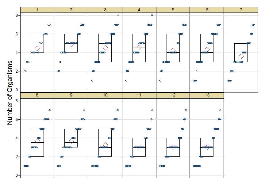
This is largely a footnote to @kjetil's answer, with which I tend to agree. But I have an extra graph that says a little more and that won't fit into a comment.
This is a combination plot. For each group, there is a quantile plot showing the detail for each group, a superimposed box showing median and quartiles in standard form and finally a diamond showing the mean, shown large for clarity. The picture is essentially one of fairly constant scatter, near symmetry and a lack of outliers or other pathological or unusual structure. I would be happy to see an ANOVA in these cases.
That said, I wouldn't expect that Poisson regression would perform badly or misleadingly for such data, provided that there was some careful handling of the variance-mean structure (e.g. in the standard error calculation).
Presumably there are (or should be) other biological and/or environmental predictors that would appear in a complete analysis.


