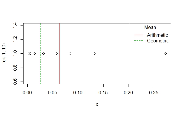
The main purpose of linear regression is to estimate a mean difference of outcomes comparing adjacent levels of a regressor. There are many types of means. We are most familiar with the arithmetic mean.
$$AM(X) = \frac{\left( X_1 + X_2 + \ldots + X_n \right)}{n}$$
The AM is what is estimated using OLS and untransformed variables. The geometric mean is different:
$$GM(X) = \sqrt[\LARGE{n}]{\left( X_1 \times X_2 \times \ldots \times X_n \right)} = \exp(AM(\log(X))$$

Practically a GM difference is a multiplicative difference: you pay X% of a premium in interest when assuming a loan, your hemoglobin levels decrease X% after starting metformin, the failure rate of springs increase X% as a fraction of the width. In all of these instances, a raw mean difference makes less sense.
Log transforming estimates a geometric mean difference. If you log transform an outcome and model it in a linear regression using the following formula specification: log(y) ~ x, the coefficient $\beta_1$ is a mean difference of the log outcome comparing adjacent units of $X$. This is practically useless, so we exponentiate the parameter $e^{\beta_1}$ and interpret this value as a geometric mean difference.
For instance, in a study of HIV viral load following 10 weeks administration of ART, we might estimate prepost geometric mean of $e^{\beta_1} = 0.40$. That means whatever the viral load was at baseline, it was on average 60% lower or had a 0.6 fold decrease at follow-up. If the load was 10,000 at baseline, my model would predict it to be 4,000 at follow-up, if it were 1,000 at baseline, my model would predict it to be 400 at follow-up (a smaller difference on the raw scale, but proportionally the same).
This is an important distinction from other answers:
The convention of multiplying the log-scale coefficient by 100 comes from the approximation $\log(x) \approx 1-x$ when $1-x$ is small. If the coefficient (on the log scale) is say 0.05, then $\exp(0.05) \approx 1.05$ and the interpretation is: a 5% "increase" in the outcome for a 1 unit "increase" in $X$. However, if the coefficient is 0.5 then $\exp(0.5) = 1.65$ and we interpret this as a 65% "increase" in $Y$ for a 1 unit "increase" in $X$. It is NOT a 50% increase.
Suppose we log transform a predictor: y ~ log(x, base=2). Here, I am interested in a multiplicative change in $x$ rather than a raw difference. I now am interested in comparing participants differing by 2 fold in $X$. Suppose for instance, I am interested in measuring infection (yes/no) following exposure to blood-borne pathogen at various concentrations using an additive risk model. The biologic model may suggest that risk increases proportionately for every doubling of concentration. Then, I do not transform my outcome, but the estimated $\beta_1$ coefficient is interpreted as a risk difference comparing groups exposed at two-fold concentration differences of infectious material.
Lastly, the log(y) ~ log(x) simply applies both definitions to obtain a multiplicative difference comparing groups differing multiplicatively in exposure levels.

