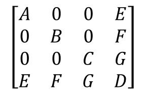
Because this is a covariance matrix, $e=h$, $f=l$, $g=m$, and $A,B,C,D$ are all positive. Changing notation to handle a generalization of this problem, consider the symmetric matrix
$$\mathbb{A} = \pmatrix{
\sigma_1^2 & 0 & 0 & \cdots & x_1 \sigma_1 \sigma_n \\
0 & \sigma_2^2 & 0 & \cdots & x_2 \sigma_2 \sigma_n \\
0 & 0 & \sigma_3^2 & \cdots & x_3 \sigma_3 \sigma_n \\
\vdots & \vdots & \vdots & \ddots& \vdots \\
x_1 \sigma_1 \sigma_n & x_2 \sigma_2 \sigma_n & x_3 \sigma_3\sigma_n &\cdots &\sigma_n^2}.$$
By comparing this to the question it is apparent that $n=4$, $\sigma_1 = \sqrt{A}$, $\sigma_2 = \sqrt{B}$, $\sigma_3 = \sqrt{C}$, $\sigma_4=\sigma_n=\sqrt{D}$, and $x_1 = e/(\sigma_1\sigma_n)$ etc. There are $n-1$ such $x_i$.
It is evident that
$$\mathbb{A} = \mathbb{U}\mathbb{X}\mathbb{U}$$
where $\mathbb{U}$ is the diagonal matrix with entries $(\sigma_1, \sigma_2, \ldots, \sigma_n)$ and (therefore)
$$\mathbb{X} = \pmatrix{
1 & 0 & 0 & \cdots & x_1 \\
0 & 1 & 0 & \cdots & x_2 \\
0 & 0 & 1 & \cdots & x_3 \\
\vdots & \vdots & \vdots & \ddots & \vdots \\
x_1 & x_2 & x_3 & \cdots & 1}.$$
It is straightforward to demonstrate (inductively) that $\mathbb{X}$ is invertible if and only if $x_1^2 + x_2^2 + \cdots + x_{n-1}^2 \ne 1$. In this case set
$$\Delta = \det(\mathbb{X}) = 1 - (x_1^2 + x_2^2 + \cdots + x_{n-1}^2)$$
and observe (using, for instance, the block-matrix formulae in Glen_b's answer) that
$$\mathbb{X}^{-1} = \frac{1}{\Delta}\pmatrix{
\Delta + x_1^2 & x_1 x_2 & x_1 x_3 & \cdots & -x_1 \\
x_2 x_1 & \Delta + x_2^2 & x_2 x_3 & \cdots & -x_2 \\
x_3 x_1 & x_3 x_2 & \Delta + x_3^2 & \cdots & -x_3 \\
\vdots & \vdots & \vdots & \ddots & \vdots \\
-x_1 & -x_2 & -x_3 & \cdots & 1}.$$
The computation of $\mathbb{U}^{-1}$ is simple--invert each of its diagonal entries--and the subsequent construction of
$$\mathbb{A}^{-1} = \mathbb{U}^{-1} \mathbb{X}^{-1} \mathbb{U}^{-1}$$
is equally easy.
To illustrate this algorithm, here is an R implementation. It creates a random symmetric matrix with positive diagonal entries and arbitrary values in the last row and column, inverts it with the algorithm, multiplies that by the original, and compares the result to the identity matrix. The arguments to the inversion function are the vector of $n$ diagonal elements a and the vector of $n-1$ elements in the bottom row of $\mathbb{X}$. Thus $\mathbb{X}$ never actually needs to be constructed.
The timing is a little slower than just using the sparseMatrix class in the Matrix package, because only native R operations (such as outer and t) are employed and these are not optimized for speed. Because the resulting inverse matrix is anything but sparse, there appears to be no inherent advantage to using sparse matrix calculations.
invert <- function(a, y) {
  n <- length(a)    # The diagonal elements
  sigma <- sqrt(a)
  x <- (y / (sigma[-n] * sigma[n]))
  Delta <- 1 - sum(x*x)
  X.inv <- outer(c(x, -1), c(x, -1)) + diag(c(rep(Delta, n-1), 0))
  X.inv <- t(t(X.inv) / sigma) / sigma
  return (X.inv / Delta)
}
#
# Create a matrix.
#
n <- 4000
a <- rexp(n)
y <- rnorm(n-1)

X <- diag(a)
n <- length(a)
X[-n, n] <- X[n, -n] <- y
#
# Invert it with the algorithm.
#
system.time(X.inv <- invert(a, y))
#
# Check that it is the inverse.
#
if (n <= 1000) {
  One <- zapsmall(X %*% X.inv)
  if(!all.equal(One, diag(rep(1,n))))
    warning("Not an inverse!") else
      message("Inverse is correct.")
}
To use the sparse-matrix solver, access the solve function in the Matrix library. Here is an illustration that continues the preceding code.
library(Matrix)
i <- c(1:n, 1:(n-1), rep(n, n-1))
j <- c(1:n, rep(n, n-1), 1:(n-1))
X.0 <- sparseMatrix(i, j, x=c(a, y, y))
system.time(X.0.inv <- solve(X.0))

