By "fitting distribution to the data" we mean that some distribution (i.e. mathematical function) is used as a model, that can be used to approximate the empirical distribution of the data you have. If you are fitting distribution to the data, you need to infer the distribution parameters from the data. You can do this by using some software that will do this for you automatically (e.g. fitdistrplus in R), or by calculating it by hand from your data, e.g using maximum likelihood (see relevant entry in Wikipedia about Poisson distribution).
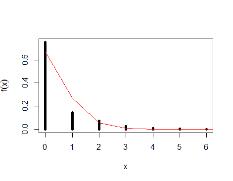
On the plot below you can see your data plotted with fitted Poisson distribution. As you can see, the line doesn't fit perfectly, as it is only an approximation.

Among other methods, one of the approaches to this problem is to use maximum likelihood. Recall that likelihood is a function of parameters for the fixed data and by maximizing this function we can find "most likely" parameters given the data we have, i.e.
$$ L(\lambda|x_1,\dots,x_n) = \prod_i f(x_i|\lambda) $$
where in your case $f$ is Poisson probability mass function. The direct, numerical way to find appropriate $\lambda$ would be to use optimization algorithm. For this first you define the likelihood function and then ask the algorithm to find the point where the function reaches it's maximum:
# negative log-likelihood (since this algorithm looks for minimum)
llik <- function(lambda) -sum(dpois(x, lambda, log = TRUE)*y)
opt.fit <- optimize(llik, c(0, 10))$minimum
You can notice something odd about this code: I multiply dpois() by y. The data you have is provided in form of a table, where for each value of $x_i$ we have accompanying counts $y_i$, while likelihood function is defined in terms of raw data, rather than such tables. You could re-create the raw data from this values by repeating each of the $x_i$'s exactly $y_i$ times (i.e. rep(x, y) in R) and using this as input to your statistical software, but you could take more clever approach. Likelihood is a product of $f(x_i|\lambda)$. Multiplying $f(x_i|\lambda)$ for identical $x_i$'s exactly $y_i$ times is the same as taking $y_i$-th power of it: $f(x_i|\lambda)^{y_i}$. Here we are maximizing log-likelihood (see here why we take log), so $\prod_i f(x_i|\lambda)^{y_i}$ becomes: $\sum_i \log f(x_i|\lambda) \times y_i$. That is how we obtained likelihood function for tabular data.
However, there is more simple way to go. We know that empirical mean of $x$'s is the maximum likelihood estimator of $\lambda$ (i.e. it lets us to estimate such value of $\lambda$ that maximizes the likelihood), so rather than using optimization software, we can simply calculate the mean. Since you have data in form of a table with counts, the most direct way to go would be to simply use weighted mean weighted mean of $x_i$'s where $y_i$'s are used as weights.
mx <- sum(x*(y/sum(y)))
This leads to identical results as if you calculated arithmetic mean from the raw data. Both maximizing the likelihood using optimization algorithm, and taking the mean lead to almost exactly the same results:
> mx
[1] 0.3995092
> opt.fit
[1] 0.3995127
So $y$'s are not mentioned anywhere in your notes as they are created artificially as a way of storing this data in aggregated form (as a table), rather than listing all the $4075$ raw $x$'s. As showed above, you can take advantage of having data in this format.
The above procedures let you to find the "best fitting" $\lambda$ and this is how you fit distribution to the data -- by finding such parameters of the distribution, that makes it fit to the empirical data.
You commented that it is still unclear for you why $y_i$'s are considered as weights. Arithmetic mean can be considered as a special case of weighted mean where all the weights are the same and equal to $1/N$:
$$ \frac{x_1 + \dots + x_n}{N} = \frac{1}{N} \left( x_1 + \dots + x_n \right) = \frac{1}{N}x_1 + \dots + \frac{1}{N}x_n $$
Now think of how your data is stored. $x_6 = 5$ and $y_6 = 4$ means that you have four fives $ x_6 = \{5,5,5,5\} $, $x_7 = 6$ and $y_7 = 2$ means $x_7 = \{6,6\}$ etc. When you calculate mean, you first need to sum them, so: $5+5+5+5 = 5 \times 4 = x_6 \times y_6$. This leads to using counts as weights for weighted mean giving exactly the same as arithmetic mean with raw data
$$ \frac{x_1 y_1 + \dots + x_n y_n}{y_1 + \dots + y_n} = \\
\frac{x_1 y_1}{N} + \dots + \frac{x_n y_n}{N} = \\
\overbrace{ \frac{x_1}{N} + \dots + \frac{x_1}{N} }^{y_1 ~ \text{times}} +
\dots + \overbrace{ \frac{x_n}{N} + \dots + \frac{x_n}{N} }^{y_n ~ \text{times}} $$
where $N = \sum_i y_i$. The same idea was applied to the likelihood function that was weighted by counts. What could be misleading in here is that in some cases we use $x_i$ to denote $i$-th observed value of $X$, while in your case $x_i$ is a specific value of $X$ that was observed $y_i$ times. As it was said before, this is just an alternative way of storing the same data.

