Poisson Regression in R based on categorical time variables

Question

I am trying to make a prediction on the number of visitors of a website and am wondering if it can be done based only on categorical time variables. I received some guidance on how to structure my input after a question on Stack Overflow, but I still can't make predictions close to the real values, no matter what I've tried and how I've combined the data.

Here are the variables in my dataset:

• website_id

• date_int - would act as a time index

• month - would be used for seasonal effect

• type - variable derived from the response variable (number of visits), representing the size of the website by calculating an average of number of visits (ranges from 1 to 5).

• D1, D2, D3, D4, D5, D6 - variables used to capture the "seasonal effect" for the day of week.

• visits

I'm leaving also a link to a sample data in case it might be relevant: train.csv.

This is what the code I've tried in R looks like.

train = read.csv("trainData.csv", header = TRUE)
head(train)

dates <- as.factor(train$date_int)
dates

months <- as.factor(train$month)
months

model<-glm(visits ~ dates + type , train, family=poisson)
summary(model)

P = predict(model, newdata = train, type = "response")
imp = round(P)
imp

I'm new to R, but from what I've seen, all the examples, even those that should be similar (like estimating sales), use other variables beside those categorical time variables. I don't have other features to base my prediction on, so I feel the need to ask if a prediction can even be made using the input given in this situation?

Answer 1

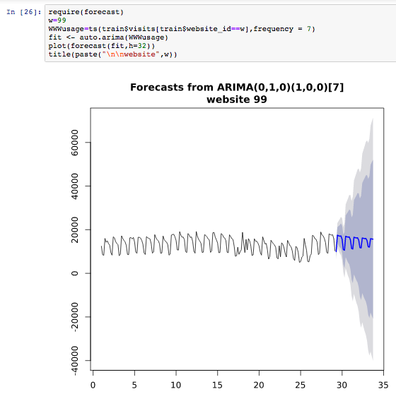
I recommend reading "Forecasting: principles and practice" https://www.otexts.org/fpp/8/2 and there are good R libs for handling your data. Using those tools, I would generate a unique forecast for each website.

require(forecast)
w=99
WWWusage=ts(train$visits[train$website_id==w],frequency = 7)
fit <- auto.arima(WWWusage)
plot(forecast(fit,h=32))    

So to build all of them:

for(w in sort(unique(train$website_id))){
    WWWusage=ts(train$visits[train$website_id==w],frequency=7)
    fit <- auto.arima(WWWusage)
    plot(forecast(fit,h=32))  
    title(paste("\n\nwebsite",w))
}

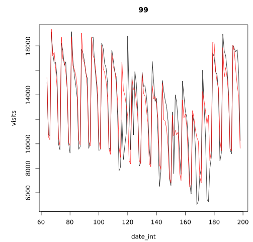
If you want to get some insight on how autoregression works, I wrote this code:

w=99
train = read.csv("/tmp/trainData.csv", header = TRUE)
train=train[train$website_id==w,]
repair=function(x) { if(length(x)==0) return(NA); return(x);}
for(b in seq(7*5,7*9,7)){
    train[[paste0('backshift',b)]]=rep(NA,nrow(train))
    for(r in 1:nrow(train)){ #slow way to do this
        train[r,paste0('backshift',b)]=repair(train$visits[train$website_id==train[r,'website_id'] 
                                          & train$date_int==(train[r,'date_int']-b)])
    }
}
train=train[complete.cases(train),]
rmse=function(x,y,k=0){
      return( sqrt(sum((x-y)^2)/(length(x)-k)))
}

require(MASS)
train$months <- as.factor(train$month)
train$date=NULL


model<-glm(visits ~. , train, family=poisson)
model=stepAIC(model,trace=F)
summary(model)

P = predict(model, newdata = train, type = "response")
imp = round(P)
rmse(imp,train$visits)
train$fit=imp
with(train[train$website_id==w,],{
    plot(date_int,visits,type='l')
    points(date_int,fit,col='red',type='l')
    title(w)
})

Here is the poisson model:

Call:
glm(formula = visits ~ date_int + D1 + D2 + D3 + D4 + D5 + D6 + 
    backshift35 + backshift42 + backshift49 + backshift56 + backshift63 + 
    months, family = poisson, data = train)

Deviance Residuals: 
    Min       1Q   Median       3Q      Max  
-72.386   -4.389    1.126    6.912   54.939  

Coefficients:
              Estimate Std. Error z value Pr(>|z|)    
(Intercept)  1.003e+01  2.405e-02 416.935  < 2e-16 ***
date_int    -3.380e-03  1.125e-04 -30.044  < 2e-16 ***
D1          -4.000e-02  3.425e-03 -11.680  < 2e-16 ***
D2           7.957e-01  9.623e-03  82.686  < 2e-16 ***
D3           6.755e-01  8.258e-03  81.800  < 2e-16 ***
D4           6.502e-01  7.997e-03  81.299  < 2e-16 ***
D5           5.791e-01  7.470e-03  77.530  < 2e-16 ***
D6           4.544e-01  6.173e-03  73.602  < 2e-16 ***
backshift35  9.173e-06  5.502e-07  16.671  < 2e-16 ***
backshift42 -1.368e-05  5.191e-07 -26.353  < 2e-16 ***
backshift49  1.408e-06  5.656e-07   2.489  0.01280 *  
backshift56 -2.305e-05  6.010e-07 -38.358  < 2e-16 ***
backshift63  1.957e-06  6.035e-07   3.242  0.00119 ** 
months9     -3.231e-01  1.332e-02 -24.258  < 2e-16 ***
months10    -2.589e-01  1.070e-02 -24.192  < 2e-16 ***
months11    -2.907e-01  7.710e-03 -37.706  < 2e-16 ***
months12    -3.915e-01  4.577e-03 -85.529  < 2e-16 ***
---
Signif. codes:  0 ‘***’ 0.001 ‘**’ 0.01 ‘*’ 0.05 ‘.’ 0.1 ‘ ’ 1

(Dispersion parameter for poisson family taken to be 1)

    Null deviance: 157970  on 134  degrees of freedom
Residual deviance:  39894  on 118  degrees of freedom
AIC: 41448

Number of Fisher Scoring iterations: 4

You can try different values of website_id (w). I had backshift start at 5 weeks ago which allows you to easily forecast 5 weeks, but you can forecast farther than that by making predictions based on predictions.