Does the order of explanatory variables matter when calculating their regression coefficients?

Question

At first I thought the order didn’t matter, but then I read about the gram-schmidt orthogonalization process for calculating multiple regression coefficients, and now I’m having second thoughts.

According to the gram-schmidt process, the later an explanatory variable is indexed among the other variables, the smaller its residual vector is because preceding variables' residual vectors are subtracted from it. As a result, the explanatory variable's regression coefficient is also smaller.

If that's true, then the residual vector of the variable in question would be larger if it were indexed earlier, since fewer residual vectors would be subtracted from it. This means that the regression coefficient would be larger too.

Ok, so I've been asked to clarify my question. So I've posted screenshots from the text that got me confused in the first place. Ok, here goes.

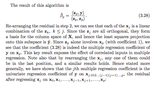
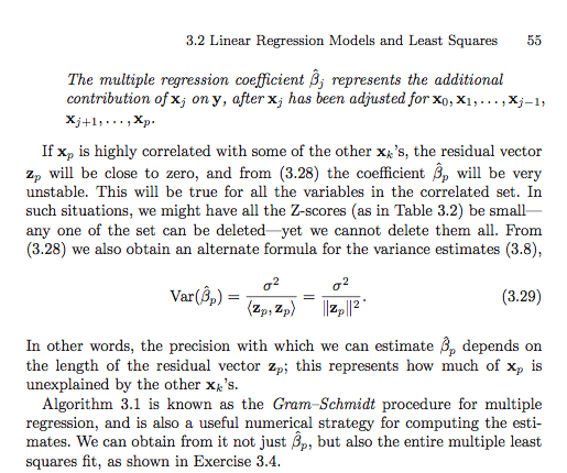
My understanding is that there are at least two options to calculate the regression coefficients. The first option is denoted (3.6) in the screenshot below.

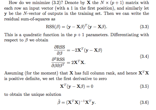
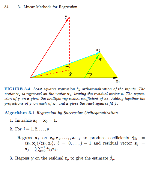
Here is the second option (I had to use multiple screenshots).

Unless I am misreading something (which is definitely possible), it seems that order matters in the second option. Does it matter in the first option? Why or why not? Or is my frame of reference so messed up that this isn't even a valid question? Also, is this all somehow related to Type I Sum of Squares vs Type II Sum of Squares?

Thanks so much in advance, I am so confused!

Answer 1

I believe the confusion may be arising from something a bit simpler, but it provides a nice opportunity to review some related matters.

Note that the text is not claiming that all of the regression coefficients $\newcommand{\bhat}{\hat{\beta}}\newcommand{\m}{\mathbf}\newcommand{\z}{\m{z}}\bhat_i$ can be calculated via the successive residuals vectors as $$ \bhat_i \stackrel{?}{=} \frac{\langle \m y, \z_i \rangle}{\|\z_i\|^2}\>, $$ but rather that only the last one, $\bhat_p$, can be calculated this way!

The successive orthogonalization scheme (a form of Gram–Schmidt orthogonalization) is (almost) producing a pair of matrices $\newcommand{\Z}{\m{Z}}\newcommand{\G}{\m{G}}\Z$ and $\G$ such that $$ \m X = \Z \G \>, $$ where $\Z$ is $n \times p$ with orthonormal columns and $\G = (g_{ij})$ is $p \times p$ upper triangular. I say "almost" since the algorithm is only specifying $\Z$ up to the norms of the columns, which will not in general be one, but can be made to have unit norm by normalizing the columns and making a corresponding simple adjustment to the coordinate matrix $\G$.

Assuming, of course, that $\m X \in \mathbb R^{n \times p}$ has rank $p \leq n$, the unique least squares solution is the vector $\bhat$ that solves the system $$ \m X^T \m X \bhat = \m X^T \m y \>. $$

Substituting $\m X = \Z \G$ and using $\Z^T \Z = \m I$ (by construction), we get $$ \G^T \G \bhat = \G^T \Z^T \m y \> , $$ which is equivalent to $$ \G \bhat = \Z^T \m y \>. $$

Now, concentrate on the last row of the linear system. The only nonzero element of $\G$ in the last row is $g_{pp}$. So, we get that $$ g_{pp} \bhat_p = \langle \m y, \z_p \rangle \>. $$ It is not hard to see (verify this as a check of understanding!) that $g_{pp} = \|\z_p\|$ and so this yields the solution. (Caveat lector: I've used $\z_i$ already normalized to have unit norm, whereas in the book they have not. This accounts for the fact that the book has a squared norm in the denominator, whereas I only have the norm.)

To find all of the regression coefficients, one needs to do a simple backsubstitution step to solve for the individual $\bhat_i$. For example, for row $(p-1)$, $$ g_{p-1,p-1} \bhat_{p-1} + g_{p-1,p} \bhat_p = \langle \m z_{p-1}, \m y \rangle \>, $$ and so $$ \bhat_{p-1} = g_{p-1,p-1}^{-1} \langle \m z_{p-1}, \m y \rangle \> - g_{p-1,p-1}^{-1} g_{p-1,p} \bhat_p . $$ One can continue this procedure working "backwards" from the last row of the system up to the first, subtracting out weighted sums of the regression coefficients already calculated and then dividing by the leading term $g_{ii}$ to get $\bhat_i$.

The point in the section in ESL is that we could reorder the columns of $\m X$ to get a new matrix $\m X^{(r)}$ with the $r$th original column now being the last one. If we then apply Gram–Schmidt procedure on the new matrix, we get a new orthogonalization such that the solution for the original coefficient $\bhat_r$ is found by the simple solution above. This gives us an interpretation for the regression coefficient $\bhat_r$. It is a univariate regression of $\m y$ on the residual vector obtained by "regressing out" the remaining columns of the design matrix from $\m x_r$.

General QR decompositions

The Gram–Schmidt procedure is but one method of producing a QR decomposition of $\m X$. Indeed, there are many reasons to prefer other algorithmic approaches over the Gram–Schmidt procedure.

Householder reflections and Givens rotations provide more numerically stable approaches to this problem. Note that the above development does not change in the general case of QR decomposition. Namely, let $$ \m X = \m Q \m R \>, $$ be any QR decomposition of $\m X$. Then, using exactly the same reasoning and algebraic manipulations as above, we have that the least-squares solution $\bhat$ satisfies $$ \m R^T \m R \bhat = \m R^T \m Q^T \m y \>, $$ which simplifies to $$ \m R \bhat = \m Q^T \m y \> . $$ Since $\m R$ is upper-triangular, then the same backsubstitution technique works. We first solve for $\bhat_p$ and then work our way backwards from bottom to top. The choice for which QR decomposition algorithm to use generally hinges on controlling numerical instability and, from this perspective, Gram–Schmidt is generally not a competitive approach.

This notion of decomposing $\m X$ as an orthogonal matrix times something else can be generalized a little bit further as well to get a very general form for the fitted vector $\hat{\m y}$, but I fear this response has already become too long.

Answer 2

I had a look through the book and it looks like exercise 3.4 might be useful in understanding the concept of using GS to find all the regression coefficients $\beta_j$ (not just the final coefficient $\beta_p$ - so I typed up a solution. Hope this is useful.

Exercise 3.4 in ESL

Show how the vector of least square coefficients can be obtained from a single pass of the Gram-Schmidt procedure. Represent your solution in terms of the QR decomposition of $X$.

Solution

Recall that by a single pass of the Gram-Schmidt procedure, we can write our matrix $X$ as $$X = Z \Gamma,$$ where $Z$ contains the orthogonal columns $z_j$, and $\Gamma$ is an upper-diagonal matrix with ones on the diagonal, and $\gamma_{ij} = \frac{\langle z_i, x_j \rangle}{\| z_i \|^2}$. This is a reflection of the fact that by definition, $$ x_j = z_j + \sum_{k=0}^{j-1} \gamma_{kj} z_k. $$

Now, by the $QR$ decomposition, we can write $X = QR$, where $Q$ is an orthogonal matrix and $R$ is an upper triangular matrix. We have $Q = Z D^{-1}$ and $R = D\Gamma$, where $D$ is a diagonal matrix with $D_{jj} = \| z_j \|$.

Now, by definition of $\hat \beta$, we have $$ (X^T X) \hat \beta = X^T y. $$ Now, using the $QR$ decomposition, we have \begin{align*} (R^T Q^T) (QR) \hat \beta &= R^T Q^T y \\ R \hat \beta &= Q^T y \end{align*}

$R$ is upper triangular, we can write \begin{align*} R_{pp} \hat \beta_p &= \langle q_p, y \rangle \\ \| z_p \| \hat \beta_p &= \| z_p \|^{-1} \langle z_p, y \rangle \\ \hat \beta_p &= \frac{\langle z_p, y \rangle}{\| z_p \|^2} \end{align*} in accordance with our previous results. Now, by back substitution, we can obtain the sequence of regression coefficients $\hat \beta_j$. As an example, to calculate $\hat \beta_{p-1}$, we have \begin{align*} R_{p-1, p-1} \hat \beta_{p-1} + R_{p-1,p} \hat \beta_p &= \langle q_{p-1}, y \rangle \\ \| z_{p-1} \| \hat \beta_{p-1} + \| z_{p-1} \| \gamma_{p-1,p} \hat \beta_p &= \| z_{p-1} \|^{-1} \langle z_{p-1}, y \rangle \end{align*} and then solving for $\hat \beta_{p-1}$. This process can be repeated for all $\beta_j$, thus obtaining the regression coefficients in one pass of the Gram-Schmidt procedure.

Answer 3

Why not try it and compare? Fit a set of regression coefficients, then change the order and fit them again and see if they differ (other than possible round-off error).

As @mpiktas points out it is not exactly clear what you are doing.

I can see using GS to solve for $B$ in the least squares equation $(x'x)B=(x'y)$. But then you would be doing the GS on the $(x'x)$ matrix, not the original data. In this case the coefficients should be the same (other than possible rounding error).

Another approach of GS in regression is to apply GS to the predictor variables to eliminate colinearity between them. Then the orthogonalized variables are used as the predictors. In this case order matters and the coefficients will be different because the interpretation of the coefficients depends on the order. Consider 2 predictors $x_1$ and $x_2$ and do GS on them in that order then use as predictors. In that case the first coefficient (after the intercept) shows the effect of $x_1$ on $y$ by itself and the second coefficient is the effect of $x_2$ on $y$ after adjusting for $x_1$. Now if you reverse the order of the x's then the first coefficient shows the effect of $x_2$ on $y$ by itself (ignoring $x_1$ rather than adjusting for it) and the second is the effect of $x_1$ adjusting for $x_2$.