I'm having a hard time understanding the reasoning behind it. Imagining the case of a single independent variable, if the correlation between it and the dependent is very negative, a nonlinear least squares would find a really poor fit. In the multidimensional case, wouldn't applying the constraint then similarly risk finding a very poor fit? If the data truly calls for some negative slopes? It almost seems like one should use regular least squares and if a coefficient is counterintuitively negative then check for errors in assumptions or possibly drop it rather than try and mask it by forcing a constraint? Isn't doing that similar to excluding random observations in analysis to get a prettier summary instead of explaining it?
-
$\begingroup$ I'll do you one better. Suppose you are trying to do a least squares fit to find the closest covariance matrix C to a matrix M which is not positive semi-definite. In such case, your optimization problem includes the constraint $C \succeq 0$, which specifies that C must be a symmetric positive semi-definite matrix. Would it make sense to find a covariance matrix which isn't symmetric positive definite? By omitting that constraint, you can get a better match, but it's not meaningful. Nonnegativity constraints serve to constrain an optimization problem. Use whatever constraints make sense. $\endgroup$– Mark L. StoneCommented May 12, 2016 at 1:47
2 Answers
I get to use non-negative least-squares fit in cases with many correlated independent variables which should not be negative (the model is obviously strictly addition and does not allow subtraction, because it would not make physical sense) where the correlation makes that contrasts between two of those correlated variables (a differencing which means one positive and one negative variable) are sensitive to being fitted.
Example 1
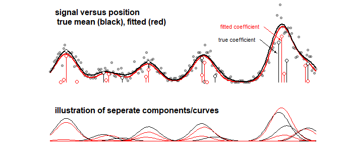
See for instance the following type of fit from this question: Why doesn't collinearity affect the predictions?

This image represents the fitting of a curve as a sum of different components. There are many of these components. If you would not use non-negative least squares then you would create the possibility for those components to become negative which might be in particular cases be unphysical.
The reason for the tendency of a model to introduce negative components would be because that the difference between two components (which means one positive and one negative) might happen to reduce some particular residuals. (so it might be subtle and does not neccesarily mean a bad fit)
Example 2
Say you wish to blend wines together in order to create some desirable profile. You try to find an optimal mixture with a fitting method where you have a number of $n$ wines, $x_1, x_2, ..., x_n$ that you can mix together and you desire to get some profile $y$ out of it.
You could obtain an optimal mixture by optimizing some cost function, e.g. least squares.
It could be the case that two wines are different in only one feature. Say wine 1 is sweeter than wine 2.
Then mathematically you could make your blend of wines less sweet, without changing other aspects, by adding more of wine 2 and subtracting wine 1. But obviously this makes no physical sense. You can not subtract a wine from a blend.
Thus in such a case, where parameters need to be strictly positive, it is useful to impose boundaries on the parameters.
This does not mean that you are gonna make a bad fit. You may get a sufficiently fine fit with positive coefficients. It means that you are not gonna fit into an unphysical realm, in order to make only slight improvements.
(in regularized regression you actually have this penalized, and increasing the magnitude of coefficients for only slight improvements will not happen easily, but with straightforward non-negative least squares you may get into this situation easily)
Numerical example
          sugar  acid  alcohol   fruity  flowery  intensity
wine 1    1      1      2        3       2        5
wine 2    2      1      2        3       2        5
wine 3    1      3      5        1       3        1
wine 4    4      4      1        2       4        3

target    3      2      2        2       3        2
Say we try to optimize target profile with least-squares...
then we get for NNLS a sum of 0.17 wine2 + 0.20 wine3 + 0.47 wine4 which gives the profile
           sugar  acid  alcohol   fruity  flowery  intensity
 target    3      2      2        2       3        2
 nnls      2.41   2.64   1.82     1.65    2.82     2.46
which is reasonable
with regular least squares we make a sum of -0.94 wine1 + 1.14 wine2 + 0.26 wine3 + 0.35 wine4
           sugar  acid  alcohol   fruity  flowery  intensity
 target    3      2      2        2       3        2
 ls        3      2.37   2.05     1.57    2.58     2.33
which is better, and especially on sugar/sweetness.
So we are using the difference of wine1 and wine2 to improve the fit, but it would not make sense to add more of wine2 and subtract wine1 in order to make the blend more sweet, because there is physically not such thing as subtracting.
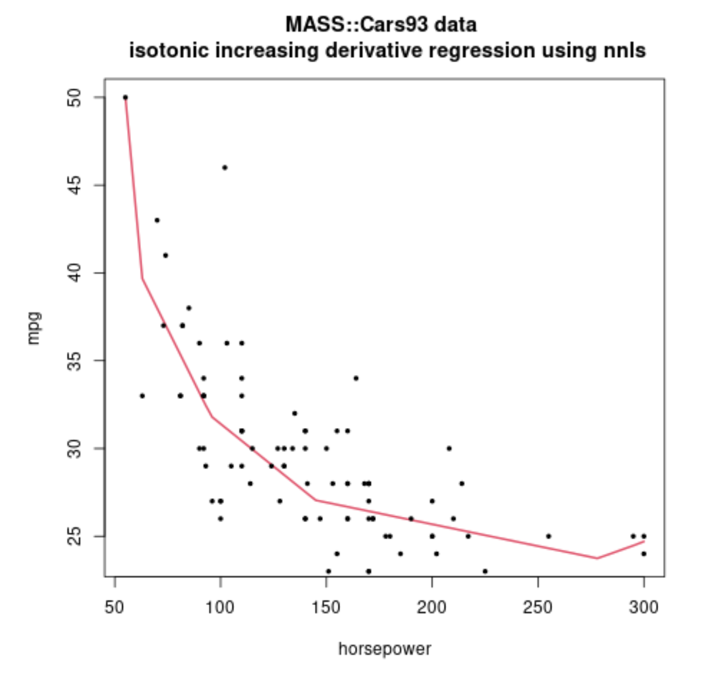
Isotonic regression
Another way to use nnls is in isotonic regression. Where the regressor matrix is composed of stepfunctions or ReLU terms.
Example:
library(nnls)
library(MASS)

### some data
data <- list(x=Cars93$Horsepower,
             y=Cars93$MPG.highway)
### order data, useful later for plotting
data$y = data$y[order(data$x)]
data$x = data$x[order(data$x)]


### isotonic regression using non-negative least squares regression
### we use a simple regression with fixed knots positions
n = 500
breaks2 = unique(quantile(data$x, probs = seq(0,1,length.out = n+1)))

l2 = length(breaks2)

### generate a regressor matrix
mX  = 0*data$x+1 ### intercept term
mX  = cbind(mX,-(data$x-data$x[1])) ###  initial negative slope
for (i in 3:l2) {
  new_vec = (data$x>breaks2[i])*(data$x-breaks2[i])
  mX = cbind(mX,new_vec)
}

### the regression
y = data$y
modstart = nnls(mX, y)

### plotting
plot(data$x,modstart$fitted,col=2, lwd = 2, type = "l",
     xlab = "horsepower", ylab = "mpg")
points(data$x,data$y, pch = 19, col = 1, cex = 0.5)
title("MASS::Cars93 data \n isotonic increasing derivative regression using nnls")
-
1$\begingroup$ The wine example is easy to understand. Just what I was looking for. $\endgroup$ Commented Jun 15, 2020 at 16:31
-
$\begingroup$ So, this means that it never allowed the weights to go negative right? $\endgroup$– Worthy7Commented Apr 23, 2023 at 5:14
-
1$\begingroup$ @Worthy7 I am not sure what you mean by 'it never allowed'. By definition the end result is with non-negative weights. If you refer by 'it' to the algorithm that does the fitting and 'never' not any time during the steps of the algorithm, then depending on the algorithm you may have states with negative weights. An example is given here: How do Lawson and Hanson solve the unconstrained least squares problem? (The negative coefficients occur in the
feasible_setfunction). $\endgroup$ Commented Apr 23, 2023 at 7:12
A typical situation is when the unknown parameters are a probability vector: $$ p_i > 0,\sum_i p_i = 1, $$ whereas the data are know function thereof, e.g., $$ \pi_\alpha = \sum_i W_{\alpha i} p_i. $$ E.g., $p_i$ could be the unknown concentrations of chemical compounds in a rock, while $\pi_\alpha$ are the mass, density and other measurable characteristics.
We then can try to estimate the concentrations by minimizing $$ \left(\pi_\alpha - \sum_i W_{\alpha i} p_i\right)^2 $$ subject to the constraint that $p_i$ are positive and sum up to one, which is a constrained non-negative least squares problem.

