8
$\begingroup$

In the commonly mentioned mammography screening problem with a screening likelihood of 80%, a prior of 10% and a false positive rate of 50%, or its variants, it is easy to explain that the conditional posterior probability that a positive screening indicates a cancer is present is only 15%. This is most easily shown by counts, with an n = 1000, true cancer cases = 100, cancers detected = 80, and false positives = 450. Then the probability that a positive screening indicates a cancer present is true positives / (true positives + false positives) or 80 / (100 + 450) = 0.145 or 15%.

The intuition is that the true positives are conditioned on the sum of the true and false positives because the sum of the true and false positives constitute a subset of all results. This is because the false negatives and true negatives are excluded from the calculation, and so the conditional set is a subset.

If we shift the problem to the continuous case with a binomial likelihood and a beta prior, then the normalizing constant becomes an integral, as for the true positives term (p = proportion)

$$\int_0^1 {\left( {\begin{array}{*{20}{c}}n\\x\end{array}} \right)p_{}^x{{(1 - p)}^{n - x}}\frac{{\Gamma (a + b)}}{{\Gamma (a)\Gamma (b)}}p_{}^{a - 1}{{(1 - {p_{}})}^{b - 1}}} dp % MathType!MTEF!2!1!+- % feaagKart1ev2aaatCvAUfeBSjuyZL2yd9gzLbvyNv2CaerbuLwBLn % hiov2DGi1BTfMBaeXatLxBI9gBaerbd9wDYLwzYbItLDharqqtubsr % 4rNCHbGeaGqiVu0Je9sqqrpepC0xbbL8F4rqqrFfpeea0xe9Lq-Jc9 % vqaqpepm0xbba9pwe9Q8fs0-yqaqpepae9pg0FirpepeKkFr0xfr-x % fr-xb9adbaqaaeGaciGaaiaabeqaamaabaabaaGcbaaeaaaaaaaaa8 % qadaWdXaqaamaabmaapaqaauaabeqaceaaaeaapeGaamOBaaWdaeaa % peGaamiEaaaaaiaawIcacaGLPaaacaWGWbWaa0baaSqaaaqaaiaadI % haaaGccaGGOaGaaGymaiabgkHiTiaadchacaGGPaWaaWbaaSqabeaa % caWGUbGaeyOeI0IaamiEaaaak8aadaWcaaqaaiabfo5ahjaacIcaca % WGHbGaey4kaSIaamOyaiaacMcaaeaacqqHtoWrcaGGOaGaamyyaiaa % cMcacqqHtoWrcaGGOaGaamOyaiaacMcaaaWdbiaadchadaqhaaWcba % aabaGaamyyaiabgkHiTiaaigdaaaGccaGGOaGaaGymaiabgkHiTiaa % dchadaWgaaWcbaaabeaakiaacMcadaahaaWcbeqaaiaadkgacqGHsi % slcaaIXaaaaaqaaiaaicdaaeaacaaIXaaaniabgUIiYdGccaWGKbGa % amiCaaaa!6018! $$

and a similar term for the false positives.

What is not clear however, it how to restate the idea of a subset in the continuous case, and I can find no one who does this. Rather one finds language that either 1) this integral gives the constant to make the calculation needed to have a probability distribution defined on the [0, 1] interval, or 2) that proportionality is invoked and the value of the integral is not needed to find the posterior, especially using MCMC, or 3) the integral is the probability of the evidence. This last explanation seems closer to the idea of a subset, but it is not clearly and explicitly connected.

I am writing an intuitive introduction to Bayes’ theorem, and want to continue the intuitive idea of a subset for the conditional probability that defines the posterior. So I need language to explain how this integral is just the continuous restatement of the subset in the discrete numbers case.

Any suggestions?

$\endgroup$
1

3 Answers 3

4
$\begingroup$

I needed to do this for a course I'm preparing, so I created this demonstration website: A demonstration of Bayes' theorem as "selecting a subset" in the binomial case (make sure to hide the toolbars, bottom right). Basically, if you show the joint distribution -- which is just $p(y\mid\theta)p(\theta)$ -- you can see the "subsets" of the joint distribution that you need to select, which are those $\theta$ values that correspond to $Y=y$ (whatever you observed).

The source code for that page can be found here: Rmarkdown source for page.

(I used $\theta$ for the binomial probability instead of $p$ because $p(p)$ looks confusing...)

$\endgroup$
0
4
$\begingroup$

Besides the interpretations you mention, you can think of the normalizing constant as the value of the prior predictive distribution at the observed x. If the prior predictive is discrete then this is a probability mass, and if the prior predictive is continuous it is a probability density.

The prior predictive is in the continuous case is $$ p(x) = \int_\Theta p(\theta)p(x|\theta) $$

Which is a distribution that assigns probability mass/density to the outcomes in the sample space. Then when x is observed it is fixed at the observed x and fits in the denominator of Bayes' theorem.

However, note that with continuous distributions there is no mathematical constraint on the density value assigned to a set with measure zero (i.e., zero probability), and since any specific point on a continuous distribution indeed has measure zero then technically the value of the density on the prior predictive at exactly x can be set arbitrarily. But that aside, I think this way of visualizing the normalizing constant is fairly intuitive.

You can read more here. (Let me know if you don't have access) This too, which is a bit more modern.

$\endgroup$
1
$\begingroup$

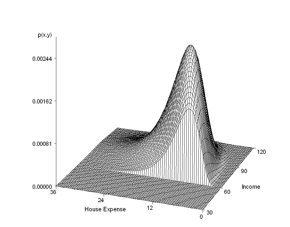
Richard's 3-d graphic was very helpful. What I need, however, is something I can paste as graph in a manuscript. After some searching, I located this image from Westfall and Henning, Understanding Advanced Statistical Methods, Chapman & Hall/CRC, 2013.

enter image description here

Relabeling the axes as the binomial probability p on the left and the number of successes y on the right then illustrates a binomial distribution, and the face of the joint distribution then is the marginal distribution to be integrated.

Further, this joint distribution made me realize that our vocabulary for this is lacking. We use the term “marginal” for the relevant subset for the normalizing constant because that vocabulary comes from a two way contingency table with discrete data where the sum of the probabilities is written in the margins of the table. We continue to use the same vocabulary in the joint distribution continuous case, but it is not descriptive.

But the figure from Westfall and Henning makes clear that for the normalizing constant we are integrating over a “slice” of the joint distribution for the value of y, the number of successes in the binomial case. “Slice” is much clearer than marginal and this figure makes instantly clear what is the relevant subset for integration.

$\endgroup$
0

Your Answer

By clicking “Post Your Answer”, you agree to our terms of service and acknowledge you have read our privacy policy.

Not the answer you're looking for? Browse other questions tagged or ask your own question.