Out of ideas: transformation of continuous variables to obtain normality of residuals seemingly impossible

Question

I've been browsing stackexchange for days to come up with decent solutions, but to no avail so far. Some threads seem to apply and offer solutions (e.g. How to transform negative data to be homoscedastic; How should I transform non-negative data including zeros?; When to transform predictor variables when doing multiple regression?; When conducting multiple regression, when should you center your predictor variables & when should you standardize them?; Variables are often adjusted (e.g. standardised) before making a model - when is this a good idea, and when is it a bad one?; Transforming extremely skewed distributions; R: test normality of residuals of linear model - which residuals to use), but the nature of my data always puts spikes in the wheels.

I'm performing multiple regression on a set of categorical and continuous variables in order to determine which variables can explain variation in the dependent variable. One of the main challenges in the first phase of model building is to transform the continuous explanatory variables in order to achieve linear relations with the dependent variable, after all (as far as I understand) that's necessary for the model assumptions to be met. I won't even involve the categorical variables for now.

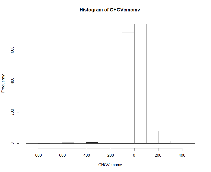
1. My dependent variable expresses the difference between empirically measured groundwater table (GWT) depths and modeled GWT depths. The difference can be either positive or negative and is not normally distributed (i.e. too heavy-tailed, I think). Not that it should be normally distributed, but it entails both positive and negative values (see infra).

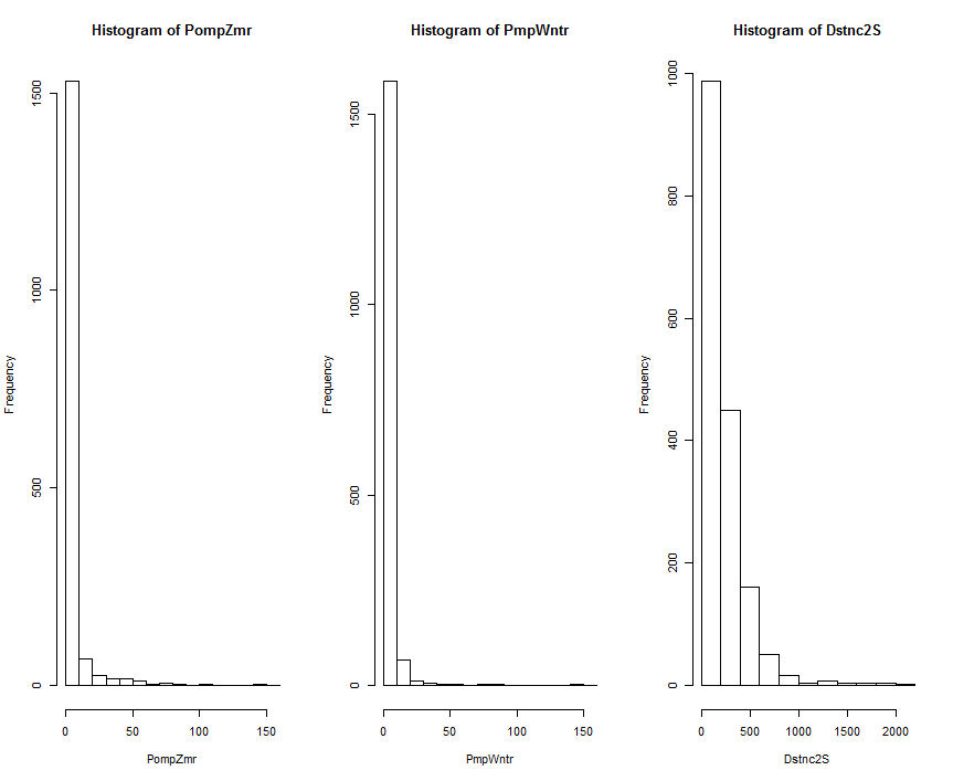
2. All independent variables are exclusively positive, but very positively skewed. Two of the independent variables correlate severely, as they express the same factor (reduction in GWT depth, in the same unit as the dependent variable: cm) measured in winter and in summer. I will have to remove one from the final model eventually as in multiple regression correlating explanatory variables should be avoided. The third explanatory variable is measured in a different scale and represents something entirely else (distance to streams, in meters).

3. Because of the different scales of the three explanatory variables, I'm inclined to standardize, but that causes the explanatory variables to have positive and negative values, like the dependent variable, and that causes problems later on (with the transformations).

4. I generally try to counter the presence of positive and negative values by applying a min-max normalization to the explanatory variables (standardized or not standardized, I tried both), normalizing the data to the interval [1-2]. I deliberately do not normalize to the interval [0-1], after all I want to be taking logarithms afterwards (see infra). This is my code:

   zDstnc2S = (Dstnc2S-mean(Dstnc2S))/sd(Dstnc2S)
   minmax_12<- function(x) (x-min(x))/(max(x) - min(x)) * (2-1)+1
   zDstnc2S_MM<-minmax_12(zDstnc2S)
   c2<-lm(GHGVcmomv~log(zDstnc2S_MM))
   shapiro.test(c2$residuals)
   

5. Positively skewed data invites the statistician to apply a log-transformation or a reciprocal transformation or a square root transformation on the data, so I've learned (Transforming extremely skewed distributions). I've run the transformations on the raw variables and on the min-maxed standardized variables. The transformations don't seem to have an effect. Is that maybe because my dependent variable is not normally distributed? Am I checking up on the effect of the transformation the wrong way? For each explanatory variable I separately run

   a<-lm(y~log(xi))
   

   and then check using

   plot(a)
   

   and

   shapiro.test(a$residuals)
   

   The W-value does not change a lot.

6. I've turned to more 'deterministic' ways of figuring out what transformation to use. I've run ggplot2 qplots on every (xi,y) combination. I've ran GAM. I've interpreted the graphical output of these tools as polynomial functions, as linear functions, as exponentials (I'm not very good at the interpretation, you've got me there - also: I would post the GAM output here but I'm only allowed to post two images here). I've tried to relate y to the xi in all of the ways mentioned in the last line. Nothing seems to improve the normality of my residuals. I've tried Box-cox, but it won't work on a dependent variable that has both positive and negative values. I've tried to run Boxcox with the min-max transformed dependent variable. Nope. Nope. Nope.

My three best guesses for the root cause of my problems are: (1) you can't effectively transform your explanatory variables to achieve normality when your dependent variable isn't normally distributed. (2) I'm checking the effectiveness of my transformations the wrong way - e.g. shapiro.test(lm$residuals) (3) I have no idea what I'm doing at all.

In case I do have to transform my dependent variable, how can I do so without losing valuable information? Remember: it's positive and negative, so @Nick Cox's cube root thing will reduce valuable information, namely that most o the yi are very close to zero. Again: I'd post the image, but after cube rooting the thing it looks like a Gaussian curve with mean 0 but it has a dip near zero, creating twin peaks ;)

I'd expand more but this post is way too long already. I suppose the answer is very simple, and I'm too silly to see it. I'll elaborate gratefully if more information is needed.

Thanks in advance.