25
$\begingroup$

Functional principal component analysis (FPCA) is something I have stumbled upon and never got to understand. What is it all about?

See "A survey of functional principal component analysis" by Shang, 2011, and I'm citing:

PCA runs into serious difficulties in analyzing functional data because of the “curse of dimensionality” (Bellman 1961). The “curse of dimensionality” originates from data sparsity in high-dimensional space. Even if the geometric properties of PCA remain valid, and even if numerical techniques deliver stable results, the sample covariance matrix is sometimes a poor estimate of the population covariance matrix. To overcome this difficulty, FPCA provides a much more informative way of examining the sample covariance structure than PCA [...]

I just don't get it. What is the drawback this paper is describing? Isn't PCA supposed to be the ultimate method to handle situations like the “curse of dimensionality”?

$\endgroup$
0

5 Answers 5

7
$\begingroup$

Exactly, as you state in the question and as @tdc puts in his answer, in case of extremely high dimensions even if the geometric properties of PCA remain valid, the covariance matrix is no longer a good estimate of the real population covariance.


There's a very interesting paper "Functional Principal Component Analysis of fMRI Data" (pdf) where they use functional PCA to visualize the variance:

...As in other explorative techniques, the objective is that of providing an initial assessment that will give the data a chance “to speak for themselves” before an appropriate model is chosen. [...]

In the paper they explain how exactly they've done it, and also provide theoretical reasoning:

The decisive advantage of this approach consists in the possibility of specifying a set of assumptions in the choice of the basis function set and in the error functional minimized by the fit. These assumptions will be weaker than the specification of a predefined hemodynamic function and a set of events or conditions as in F-masking, thus preserving the exploratory character of the procedure; however, the assumptions might remain stringent enough to overcome the difficulties of ordinary PCA.

$\endgroup$
2
  • $\begingroup$ I am struggling to understand the logic behind FPCA; I looked at the paper you cited, but still remain confused. The setting is that the data matrix is of $n\times t$ size with $n$ observed time series of length $t\gg n$. With PCA one can find the first $t$-long eigenvector of the covariance matrix; the claim is that it will be very noisy. FPCA solution is to approximate each time series with $k$ basis functions ($k\ll t$), and then perform PCA in the basis function space. Correct? If so, how is it different from smoothing each time series and then running standard PCA? Why a special name? $\endgroup$
    – amoeba
    Commented Feb 5, 2015 at 0:41
  • $\begingroup$ After reading a bit more about it, I decided to post my own answer. Perhaps you will be interested. I will certainly appreciate any additional insights. $\endgroup$
    – amoeba
    Commented Feb 6, 2015 at 13:36
30
$\begingroup$

I find "functional PCA" an unnecessarily confusing notion. It is not a separate thing at all, it is standard PCA applied to time series.

FPCA refers to the situations when each of the $n$ observations is a time series (i.e. a "function") observed at $t$ time points, so that the whole data matrix is of $n \times t$ size. Usually $t\gg n$, e.g. one can have $20$ time series sampled at $1000$ time points each. The point of the analysis is to find several "eigen-time-series" (also of length $t$), i.e. eigenvectors of the covariance matrix, that would describe "typical" shape of the observed time series.

One can definitely apply the standard PCA here. Apparently, in your quote the author is concerned that the resulting eigen-time-series will be too noisy. This can happen indeed! Two obvious ways to deal with that would be (a) to smooth the resulting eigen-time-series after PCA, or (b) to smooth the original time series before doing PCA.

A less obvious, more fancy, but almost equivalent approach, is to approximate each original time series with $k$ basis functions, effectively reducing the dimensionality from $t$ to $k$. Then one can perform PCA and obtain the eigen-time-series approximated by the same basis functions. This is what one usually sees in the FPCA tutorials. One would usually use smooth basis functions (Gaussians, or Fourier components), so as far as I can see this is essentially equivalent to the brain-dead simple option (b) above.

Tutorials on FPCA usually go into lengthy discussions of how to generalize PCA to the functional spaces of infinite dimensionality, but the practical relevance of that is totally beyond me, as in practice the functional data are always discretized to begin with.

Here is an illustration taken from Ramsay and Silverman "Functional Data Analysis" textbook, which seems to be the definitive monograph on "functional data analysis" including FPCA:
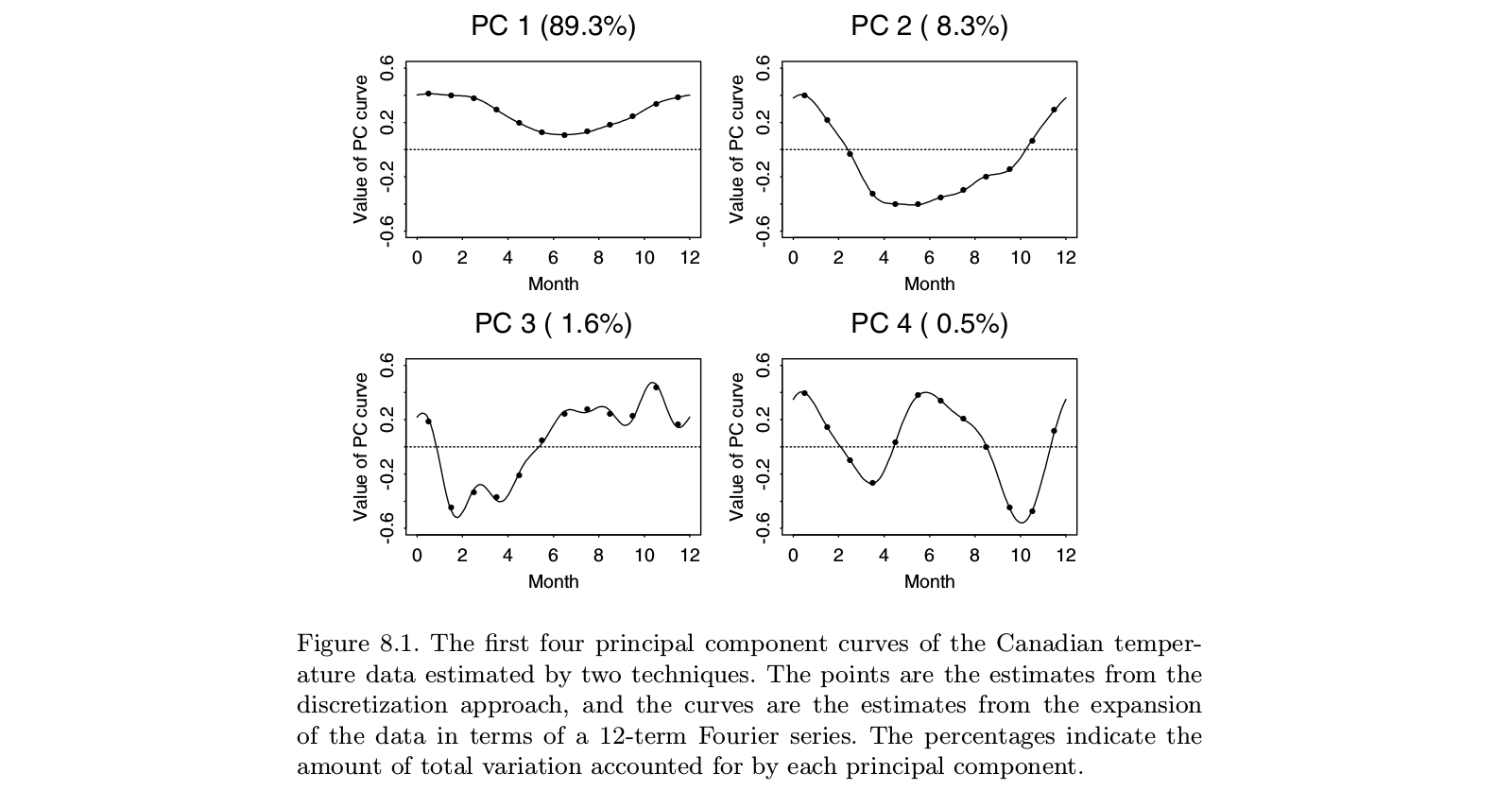
Ramsay and Silverman, FPCA

One can see that doing PCA on the "discretized data" (points) yields practically the same thing as doing FPCA on corresponding functions in Fourier basis (lines). Of course one could first do the discrete PCA and then fit a function in the same Fourier basis; it would yield more or less the same result.

PS. In this example $t=12$ which is a small number with $n>t$. Perhaps what the authors view as "functional PCA" in this case should result in a "function", i.e. "smooth curve", as opposed to 12 separate points. But this can be trivially approached by interpolating and then smoothing the resulting eigen-time-series. Again, it seems that "functional PCA" is not a separate thing, it is just an application of PCA.

$\endgroup$
4
  • 2
    $\begingroup$ In the case of sparsely irregularly sampled trajectories (eg. longitudinal data) FPCA is much more involved than "interpolating and then smoothing the resulting eigen-time-series". For example even if one somehow gets some eigencomponents calculating the projection scores of sparse data is not well-defined; see for example:Yao et al. JASA 2005. Granted for densely regularly sampled processes FPCA is effectively PCA with some smoothness penalties on top. $\endgroup$
    – usεr11852
    Commented Sep 4, 2016 at 22:37
  • 1
    $\begingroup$ Thanks, @usεr11852 (+1). I need to find time to look into it again. I will try to look up the paper you referenced and get back to this answer. $\endgroup$
    – amoeba
    Commented Sep 4, 2016 at 22:40
  • $\begingroup$ @amoeba, this all sounds almost related to discrete fourier transformation, where you recover component waves of a complex wave/time-series? $\endgroup$ Commented Oct 31, 2017 at 21:15
  • $\begingroup$ Just wondering, what interpolation methods could we use if the observation is far greater in number than t (n>>t)? Could you also elaborate on how FPCA would reduce the noise of the resulting eigen-time-series? $\endgroup$
    – son520804
    Commented Aug 19, 2020 at 15:25
15
$\begingroup$

I worked for several years with Jim Ramsay on FDA, so I can perhaps add a few clarifications to @amoeba's answer. I think on a practical level, @amoeba is basically right. At least, that's the conclusion I finally reached after studying FDA. However, the FDA framework gives an interesting theoretical insight into why smoothing the eigenvectors is more than just a kludge. It turns out that optmization in the function space, subject to an inner product that contains a smoothness penalty, gives a finite dimensional solution of basis splines. FDA uses the infinite dimensional function space, but the analysis does not require an infinite number of dimensions. It's like the kernel trick in Gaussian processes or SVM's. It's a lot like the kernel trick, actually.

Ramsay's original work dealt with situations where the main story in the data is obvious: the functions are more or less linear, or more or less periodic. The dominant eigenvectors of standard PCA will just reflect the overall level of the functions and the linear trend (or sine functions), basically telling us what we already know. The interesting features lie in the residuals, which are now several eigenvectors from the top of the list. And since each subsequent eigenvector has to be orthogonal to the previous ones, these constructs depend more and more on artifacts of the analysis and less on relevant features of the data. In factor analysis, oblique factor rotation aims to resolve this problem. Ramsay's idea was not to rotate the components, but rather to change the definition of orthogonality in a way that would better reflect the needs of the analysis. This meant that if you were concerned with periodic components, you would smooth on the basis of $D^3-D$, which eliminates sines and consines. If you wanted to remove a linear trend, you would smooth on the basis of $D^2$ which gives standard cubic splines.

One might object that it would be simpler to remove the trend with OLS and examine the residuals of that operation. I was never convinced that the value add of FDA was worth the enormous complexity of the method. But from a theoretical standpoint, it is worth considering the issues involved. Everything we do to the data messes things up. The residuals of OLS are correlated, even when the original data were independent. Smoothing a time series introduces autocorrelations that were not in the raw series. The idea of FDA was to ensure that the residuals we got from initial detrending were suited to the analysis of interest.

You have to remember that FDA originated in the early 80's when spline functions were under active study - think of Grace Wahba and her team. Many approaches to multivariate data have emerged since then - like SEM, growth curve analysis, Gaussian processes, further developments in stochastic process theory, and many more. I'm not sure that FDA remains the best approach to the questions it addresses. On the other hand, when I see applications of what purports to be FDA, I often wonder if the authors really understand what FDA was trying to do.

$\endgroup$
1
  • 1
    $\begingroup$ +1. Oops, I have noticed your answer only now, and only by chance (somebody else left a comment under my answer here and I scrolled down). Thanks a lot for contributing! I think I need to find time to do a bit more reading on this and to think about what you said about the similarity to the kernel trick. It does sound reasonable. $\endgroup$
    – amoeba
    Commented Sep 4, 2016 at 22:46
5
$\begingroup$

I'm not sure about FPCA, but one thing to remember, is that in extremely high dimensions, there is a lot more "space", and points within the space start to look uniformly distributed (i.e. everything is far from everything else). At this point the covariance matrix will start to look essentially uniform, and will be very highly sensitive to noise. It therefore becomes a bad estimate of the "true" covariance. Perhaps FPCA gets round this somehow, but I'm not sure.

$\endgroup$
1
$\begingroup$

Wikipedia has a comprehensive introduction to the functional principal component analysis. But it is too rigorous for people who have little experience in maths or statistics.

The name of functional PCA is "misleading" in some sense since theoretically, it operates on a stochastic process composed of infinite functions, rather than finite sample functions. The smoothing is a numerical "correction" for the limited samples, as well as the "discontinuous" observance across the domain in reality (for example time).

The Karhunen-Loève theory is the foundation of the functional PCA. It is an "eigendecomposition" of a covariance function of a centered, square-integrable stochastic process in $L^2$ metric space. On the other hand, PCA is an "eigendecomposition" of the variance-covariance matrix calculated from a centered finite dataset in $R^p$ metric space (p variables). Many similarities share between functional PCA and PCA once the correct "working directory" is set. So you have to figure out what is a stochastic process, what is $L^2$ metric space, in the first place. They are quite intuitionally accessible.

a funny "fact", $$ \lim \limits_{\substack{sample~size~of~functions~ \rightarrow ~\infty \\ "discontinuity"~of~f \rightarrow ~ 0} } PCA \longrightarrow fPCA $$ without smoothing.

$\endgroup$

Your Answer

By clicking “Post Your Answer”, you agree to our terms of service and acknowledge you have read our privacy policy.

Not the answer you're looking for? Browse other questions tagged or ask your own question.