The example in whuber's answer is very to the point (+1), to which I want to elaborate the rationale behind it from the theoretical perspective. For a better exposition, suppose the number of regressors is $2$ and the number of observations is $n$, so the model can be written as:
\begin{align}
y_i = \beta_0 + \beta_1X_{1, i} + \beta_2X_{2, i} + \epsilon_i, \quad
i = 1, 2, \ldots, n.
\end{align}
Further suppose the relation among $y = (y_1, \ldots, y_n)$, $X_1 = (X_{1,1}, \ldots, X_{1, n})$, $X_2 = (X_{2, 1}, \ldots, X_{2, n})$ is as set up by whuber: $X_1$ and $X_2$ are orthogonal, $y$ and $X_1$ are highly correlated, $y$ and $X_2$ are (almost) uncorrelated. We are interested in testing
The single $\beta_1$ is $0$:
\begin{align}
H_0: \beta_1 = 0 \text{ v.s. } H_1: \beta_1 \neq 0. \tag{1}
\end{align}
All $\beta$s are 0:
\begin{align}
H_0: \beta_1 = \beta_2 = 0 \text{ v.s. } H_1: \beta_1 \neq 0 \text{ or }
\beta_2 \neq 0. \tag{2}
\end{align}
It is well-known that the testing procedures applying to problem $(1)$ and $(2)$ are $t$-test and $F$-test respectively. However, the key to explain the posed paradox is recognizing the $t$-test to problem $(1)$ can also be viewed as an equivalent $F$-test, so that we are actually applying the partial $F$-test to problem $(1)$ and the overall $F$-test to problem $(2)$ respectively (a good reference to this is Applied Linear Statistical Models by Kutner et al., Section 7.3), whose testing statistics are
\begin{align}
F^{(1)} = \frac{MSR(X_1|X_2)}{MSE} = \frac{SSR(X_1, X_2) - SSR(X_2)}{MSE} \tag{3}
\end{align}
and
\begin{align}
F^{(2)} = \frac{MSR(X_1, X_2)}{MSE} = \frac{SSR(X_1, X_2)}{2MSE} \tag{4}
\end{align}
respectively. At the significance level $\alpha$, $F^{(1)}$ and $F^{(2)}$ are compared with critical points (($1 - \alpha$)-$F$-quantiles) $q_1^* = F_{1, n - 3}(1 - \alpha)$ and $q_2^*= F_{2, n - 3}(1 - \alpha)$ respectively to determine whether $H_0$ should be rejected.
Under this specific setting, it is clear that $SSR(X_2) \approx 0$, which implies that $F^{(1)}$ is approximately $2$ times of $F^{(2)}$, however, the ratio of $q_1^*$ and $q_2^*$ is less than $2$, making the null hypothesis in $(1)$ is more likely to be rejected than the null hypothesis in $(2)$: for example, if $F^{(1)}$ is slightly greater than $q_1^*$, hence the null hypothesis in $(1)$ is (barely) rejected, then $F^{(2)} \approx 0.5F^{(1)}$ is slightly greater than $0.5q_1^*$, which will be less than $q_2^*$, as it is supposed to be considerably greater than $0.5q_1^*$. Hence the null hypothesis in $(2)$ cannot be rejected at the same significance level $\alpha$.
Now let's replicate whuber's example to illustrate the above point. As can be read from the output below, $F^{(1)} = 3.012^2 = 9.072 > q_1^* = 7.597663$, $F^{(2)} = 4.684 < q_2^* = 5.420445$, hence at $\alpha = 0.01$, $H_0$ in $(1)$ is rejected but in $(2)$ is not rejected. The reason is that the ratio of $F^{(1)}$ and $F^{(2)}$ is $F^{(1)}/F^{(2)} = 1.94$, which is considerably greater than the ratio of cutoff points $q_1^*/q_2^* = 1.40$.
> set.seed(17)
> p <- 5 # Number of explanatory variables
> x <- as.matrix(do.call(expand.grid, lapply(as.list(1:p), function(i) c(-1,1))))
> y <- x[,1] + rnorm(2^p, mean=0, sd=2)
> X <- as.data.frame(x)
>
> m <- lm(y ~ Var1 + Var2, X)
> summary(m)

Call:
lm(formula = y ~ Var1 + Var2, data = X)

Residuals:
     Min       1Q   Median       3Q      Max
-3.13861 -1.34150  0.09369  1.10478  2.85457

Coefficients:
            Estimate Std. Error t value Pr(>|t|)
(Intercept)   0.5185     0.2980   1.740  0.09244 .
Var1          0.8975     0.2980   3.012  0.00534 **
Var2          0.1624     0.2980   0.545  0.58982
---
Signif. codes:  0 ‘***’ 0.001 ‘**’ 0.01 ‘*’ 0.05 ‘.’ 0.1 ‘ ’ 1

Residual standard error: 1.686 on 29 degrees of freedom
Multiple R-squared:  0.2442,    Adjusted R-squared:  0.192
F-statistic: 4.684 on 2 and 29 DF,  p-value: 0.01726

> qf(0.99, 1, 29)
[1] 7.597663
>
> qf(0.99, 2, 29)
[1] 5.420445
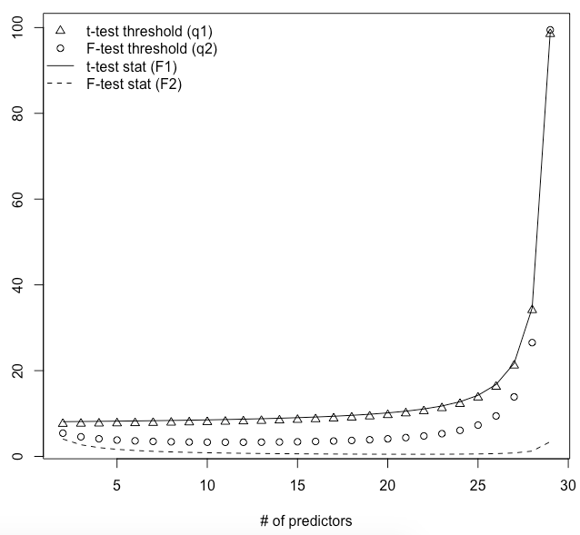
To illustrate the "insignificance of overall $F$-test inflation" effect as the number of regressors $p$, consider the same scenario as above but now $p$ ranges from $2$ to $29$ (the penultimate maximum number of regressors that $F$-test works fine).
q1 <- qf(0.99, 1, 29:2)
q2 <- qf(0.99, 2:29, 29:2)
F1 <- q1 + 0.5 # This simulates the case that t-test barely rejects H0.
F2 <- F1/(2:29) # F2 is approximately 1/p of F1 by setting.
plot(2:29, q2, xlab = "# of predictors", ylab = "")
points(2:29, q1, pch = 2)
lines(2:29, F1)
lines(2:29, F2, lty = "dashed")
legend("topleft",
       c("t-test threshold (q1)",
         "F-test threshold (q2)",
         "t-test stat (F1)",
         "F-test stat (F2)"),
       pch = c(2, 1, NA, NA),
       lty = c(NA, NA, "solid", "dashed"))
The graph is as follows. It can be seen that the dashed line is always below thresholds (hence $F$-tests are always insignificant), and as $p$ increases, the gap between the dots and the dashed line also increases, indicating that the $F$-test becomes more insignificant.


