Evaluating Forecast Errors of Exponential Smoothing Model: Is it necessary?

Question

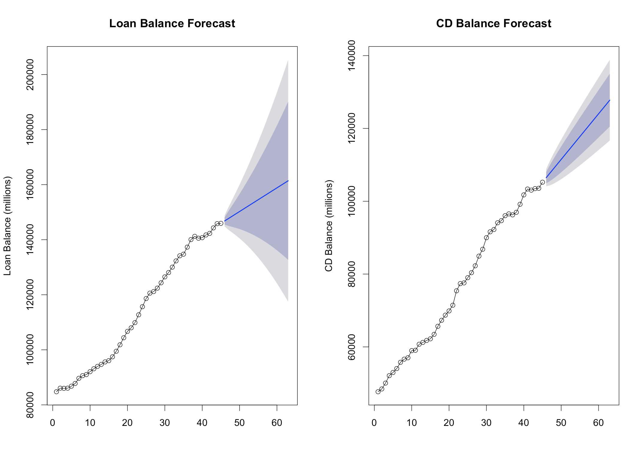
My question has to do with interpreting the ETS model that I have created using R.

To forecast this data I have used an exponential smoothing model with multiplicative errors, additive trend, and no seasonal. I am predicting 18 months into the future, and although I know this is too far in the future and terribly inaccurate, I have been asked to predict the next 18 months, so I have.

totall_ets <- ets(totals[totals$cl == "c",4], model = "ZZN")
totalcd_ets <- ets(totals[totals$cl == "l",4], model = "ZZN")
#predict 18 months past our train data
totall_fcast <- forecast(totall_ets, 18)
totalcd_fcast <- forecast(totalcd_ets, 18)

The loan balance forecast on the left is the forecast I am interested in discussing.

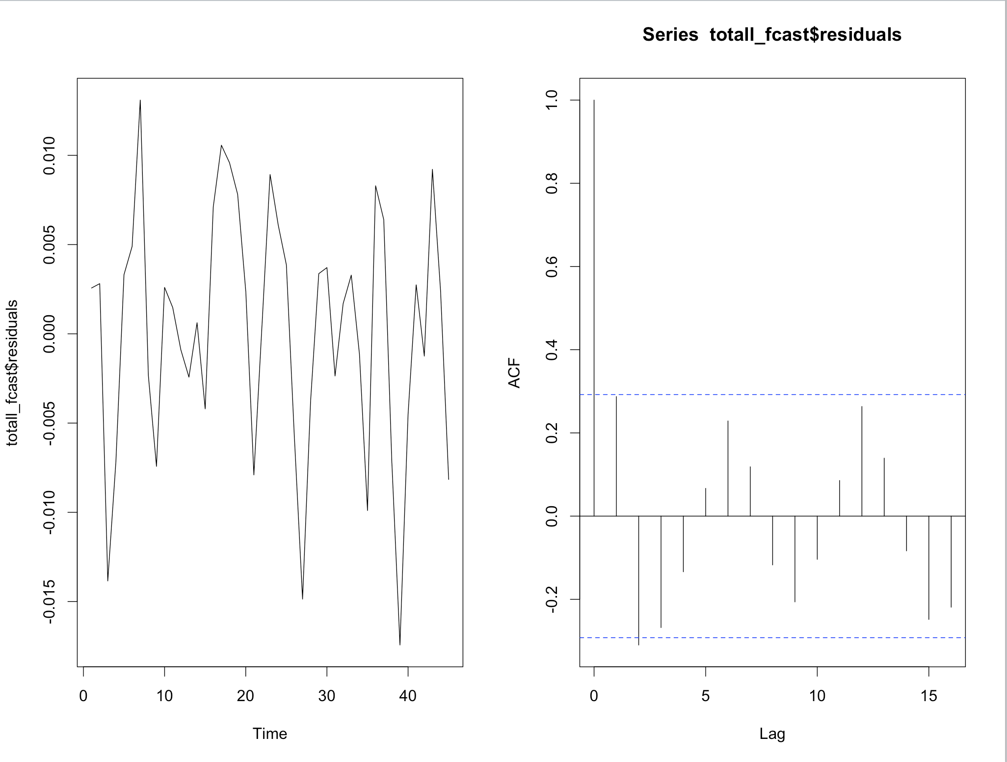
The ACF and the plotted residuals look pretty bad. The residual plots on the left show variance heteroscedasticity, and the first forecast shows a strange seasonal pattern in the acf plot.

Furthermore, the errors are clearly not normal as I've found from plotting the errors into histograms (I can't show this plot because I don't have enough reputation points to post more than two images).

Finally, the errors for my first model are not independent according to the Ljung Box Test:

Box.test(totall_fcast$residuals, lag=20, type="Ljung-Box") 
Box.test(totalcd_fcast$residuals, lag=20, type="Ljung-Box")

First forecast p-value: .0007 Second forecast p-value: .182

With all of this said, here is my question: Does it matter?

The errors are heteroscedastic, not normal, and not independent, but I am finding that the only effect is that the confidence intervals are invalid. Other than the confidence intervals, are my forecasts still satisfactory? Meaning, is there something that is ridiculous about my forecasts or is it ok because I understand and acknowledge the shortcomings of my models?

Any help will be much appreciated! ARIMA will be performed very soon to create alternative forecasts. Thank you for reading and for your help!-Tom

Answer 1

Depends how much you value the accuracy of the forecasts as to whether or not they're satisfactory. They don't look strikingly bad, but since you're likely leaving valuable information unaccounted for (i.e. heteroscedastic/correlated errors), I'd consider additional modeling and testing. I recommend trying multiple methods of modeling (looks like ARIMA and/or TBATS might be useful in this case). You could build your best ETS model and best ARIMA model and know which is best for prediction (in the past) by using time-series cross-validation. The in-sample error will not tell you that.

Oh, and you may want to test some damped trend ETS models in this case too, it often has better out-of-sample accuracy for highly trended series than non-damped, see: https://www.otexts.org/fpp/7/4