Why is correlation not very useful when one of the variables is categorical?

Question

This is a little bit of a gut check, please do help me see if I'm misunderstanding this concept, and in what way.

I have a functional understanding of correlation but I'm feeling a little grasping-at-straws to really confidently explain the principles behind that functional understanding.

As I understand it, statistical correlation (as opposed to the more general usage of the term) is a way to understand two continuous variables and the way in which they do or do not tend to rise or fall in similar ways.

The reason you can't run correlations on, say, one continuous and one categorical variable is because it's not possible to calculate the covariance between the two, since the categorical variable by definition cannot yield a mean, and thus cannot even enter into the first steps of the statistical analysis.

Is that right?

Answer 1

Correlation is the standardized covariance, i.e the covariance of $x$ and $y$ divided by the standard deviation of $x$ and $y$. Let me illustrate that.

Loosely speaking, statistics can be summarized as fitting models to data and assessing how well the model describes those data points (Outcome = Model + Error). One way to do that is to calculate the sums of deviances, or residuals (res) from the model:

$res= \sum(x_{i}-\bar{x})$

Many statistical calculations are based on this, incl. the correlation coefficient (see below).

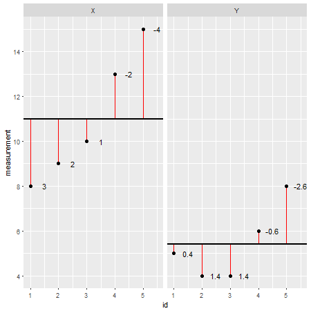
Here is an example dataset made in R (the residuals are indicated as red lines and their values added next to them):

X <- c(8,9,10,13,15)  
Y <- c(5,4,4,6,8)

By looking at each data point individually and subtracting its value from the model (e.g. the mean; in this case X=11 and Y=5.4), one could assess the accuracy of a model. One could say the model over-/ underestimated the actual value. However, when summing up all the deviances from the model, the total error tends to be zero, the values cancel each other out because there are positive values (the model underestimates a particular data point) and negative values (the model overestimates a particular data point). To solve this problem the sums of deviances are squared and now called sums of squares ($SS$):

$SS = \sum(x_i-\bar{x})(x_i-\bar{x}) = \sum(x_i-\bar{x})^2$

The sums of squares are a measure of deviation from the model (i.e. the mean or any other fitted line to a given dataset). Not very helpful for interpreting the deviance from the model (and comparing it with other models) since it is dependent on the number of observations. The more observations the higher the sums of squares. This can be taken care of by dividing the sums of square with $n-1$. The resulting sample variance ($s^2$) becomes the "average error" between the mean and the observations and is therefore a measure of how well the model fits (i.e. represents) the data:

$s^2 = \frac{SS}{n-1} = \frac{\sum(x_i-\bar{x})(x_i-\bar{x})}{n-1} = \frac{\sum(x_i-\bar{x})^2}{n-1}$

For convenience, the square root of the sample variance can be taken, which is known as the sample standard deviation:

$s=\sqrt{s^2}=\sqrt{\frac{SS}{n-1}}=\sqrt{\frac{\sum(x_i-\bar{x})^2}{n-1}}$

Now, the covariance assesses whether two variables are related to each other. A positive value indicates that as one variable deviates from the mean, the other variable deviates in the same direction.

$cov_{x,y}= \frac{\sum(x_i-\bar{x})(y_i-\bar{y})}{n-1}$

By standardizing, we express the covariance per unit standard deviation, which is the Pearson correlation coefficient $r$. This allows comparing variables with each other that were measured in different units. The correlation coefficient is a measure of the strength of a relationship ranging from -1 (a perfect negative correlation) to 0 (no correlation) and +1 (a perfect positive correlation).

$r=\frac{cov_{x,y}}{s_x s_y} = \frac{\sum(x_1-\bar{x})(y_i-\bar{y})}{(n-1) s_x s_y}$

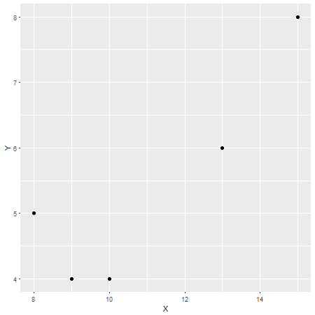
In this, case the Pearson correlation coefficient is $r=0.87$, which can be considered a strong correlation (although this is also relative depending on the field of study). To check this, here another plot with X on the x-axis and Y on the y axis:

So long story short, yes your feeling is right but I hope my answer can provide some context.

Answer 2

You are (nearly) right. Covariance (and therefore correlation too) can be computed only between numerical variables. That includes continuous variables but also discrete numerical variables.

Categorical variables could be used to compute correlation only given a useful numerical code for them, but this is not likely to get a practical advantage - maybe it could be useful for some two levels categorical variables, but other tools are likely to be more suitable.

Answer 3

There is absolutely nothing wrong with computing correlations where one of the variables is categorical. A strong positive correlation would imply that turning your categorical variable on (or off depending on your convention) causes an increase in the response. For example this could happen when calculating a logistic regression where variables are categorical: predicting the chance of a heart attack given patient comorbidities like diabetes and bmi. In this case BMI would have would have a very strong correlation with heart attacks. Would you conclude that's not useful?