How to analyze random variables with non normal distribution

Question

I'm wondering how random variables can be analyzed using parametric methods if the distribution is not normal.

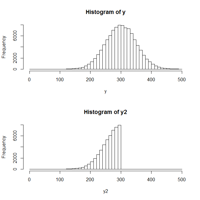
For example if a variable Y is normal distributed but I'm interested only on values Y2 which are lower than a certain limit due to agreement.

Can I use the common statistical tools to compute estimation, standard deviation, standard errors and P-values if the sample is large?

To clarify my question I created the following theoretical population:

# 100,000 values with mean 300 and sd = 50
set.seed(1234)
n <- 100000
y <- rnorm(n,300,50)

# Only y < 300 are of interest
y2 <- y[y<300]
length(y2)     # [1] 49,828

par(mfrow=c(2,1))
hist(y, breaks=seq(0,max(y)+10,10))
hist(y2, breaks=seq(0,max(y)+10,10))

# mean and sd of y
mean(y)        # 300.1465
median(y)      # 300.2244
sd(y)          # 49.97292

# mean and sd of the interested values (y2)
mean(y2)       # 260.1354
median(y2)     # 266.3348
sd(y2)         # 30.04559

Now, I make an experiment. I take a sample of $s=100$:

# Experiment:
y.exp <- sample(y,s)

# Only y<300 are of interest (for example due to a game rule)
y.int <- y.exp[y.exp<300]
mean(y.int)     # 259.3562
sd(y.int)       # 32.56482
length(y.int)   # 38

I'm interest in the following hypothesis:
$H_0: \mu_0 = 250$
$H_{alt}: \mu_0 \ne 250$

Assuming that the sample is large enough I do a t-test:

# t-test:
mu0 <- 250
t.test(y.int,mu=mu0)  # t = 1.7711, df = 37, p-value = 0.08478

Here are my questions:

1. If a sample size is large enough can I use the common statistical tools like t-test, linear regression, etc. (maybe supported by the law of large numbers)?
2. Are there alternative methods which consider special distributions (like this truncated normal distribution). I know there are non-parametric methods or truncated regression. I'm interested in parametric methods. Truncated regression answer another question: what is it the mean value of the normal distribution if the data a truncated. I'm interested in the mean value of the truncated data.
3. Does standard deviation makes sense if the underlying distribution is not normal?

Answer 1

As a complement to the short answers made in remarks, I'll illustrate the behavior of linear regression with half-normal error terms.

Here is a function for generating half-normal variables with specified mean and standard deviation.

rhnorm <- function(n, mean = 0, sd = 1)
  mean + sd/sqrt(1-2/pi)*(abs(rnorm(n))-sqrt(2/pi))

Let's simulate a simple linear model and analyze it with lm

> X <- runif(1000)
> Y <- 2 + 3*X + rhnorm(length(X), sd = 2)
> summary(lm(Y~X))

Residuals:
    Min      1Q  Median      3Q     Max 
-2.6706 -1.6689 -0.4588  1.1634  8.4628 

Coefficients:
                Estimate Std. Error t value Pr(>|t|)    
(Intercept)   2.0377     0.1251   16.29   <2e-16 ***
X             2.9564     0.2230   13.26   <2e-16 ***
---
Signif. codes:  0 ‘***’ 0.001 ‘**’ 0.01 ‘*’ 0.05 ‘.’ 0.1 ‘ ’ 1

Residual standard error: 2.032 on 998 degrees of freedom
Multiple R-squared:  0.1497,    Adjusted R-squared:  0.1489 
F-statistic: 175.7 on 1 and 998 DF,  p-value: < 2.2e-16

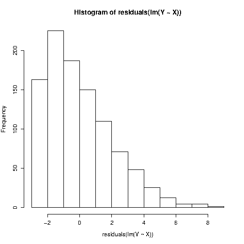
As you see, the coefficients are well estimated, as well as the residual error, and of course the residuals. The histogram of the residuals is skewed, which would wrongly lead many users to consider that they should not use linear regression (and many reviewers to tell research paper authors that they should not!).

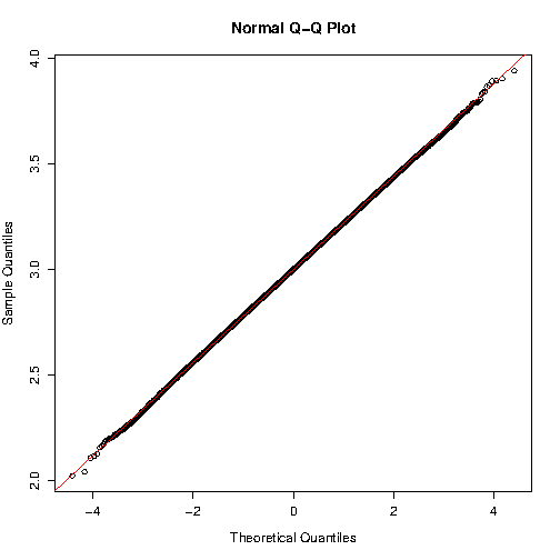
Let's explore further with simulation. First, repeat the above simulation $10^5$ times. Theory tells that the estimate of the X coefficients should be normal, with mean 3 and standard deviation $2/(\sqrt n \sigma_X)$, in our case $0.22$.

> a <- replicate( 1e5, { Y <- 2 + 3*X + rhnorm(length(X), sd = 2);
                         summary(lm(Y~X))$coefficients[2,]  } )

> mean( a[1,] )
[1] 2.999933
> sd( a[1,] )
[1] 0.2186882
> qqnorm(a[1,]); abline(3, .22, col="red")

I fail to see any problem! We can do similar simulations under the null hypothesis to be sure that there’s no gross type I error issue.

> b <- replicate( 1e5, { Y <- 2 + rhnorm(length(X), sd = 2);
                         summary(lm(Y~X))$coefficients[2,]  } )
> mean( b[1,] )
[1] -0.0002721078
> sd( b[1,] )
[1] 0.2186087

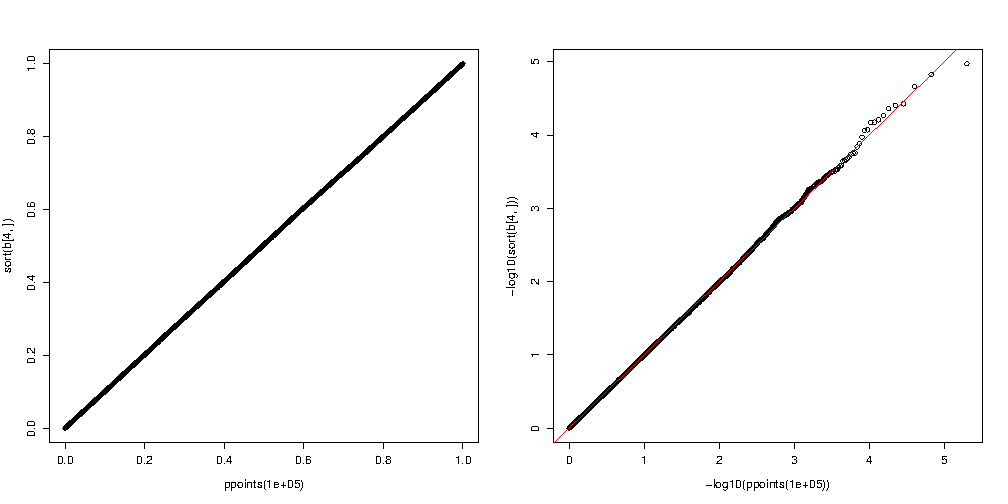
Let's so do a qq-plot of the p-values, in normal scale and in $(-\log_ {10})$-scale to have a better view on small p-values.

> par(mfrow=c(1,2))
> plot(ppoints( 1e5) , sort(b[4,]))
> plot(-log10(ppoints( 1e5)) , -log10(sort(b[4,]))); abline(0,1,col="red")

Definitely nothing’s wrong happening.

I am a lecturer, and I have tried this with my students with several distribution of the error terms. It seems that the only way to get serious problems is to use pathologically heavy tailed error terms, such as $t(1)$ (or $t(2)$ but I am not even sure of this one — try if you’re curious!).

PS Thinking about it again a little later... we have $\hat\beta = (X'X)^{-1}X'Y$. As long as $X'Y$ is approximately (multivariate) normal, everything is ok; however if some columns of $X$ are indicator functions, this could be fail e.g. if there only a few ones in the column, or if a linear combination of the columns has the same property.