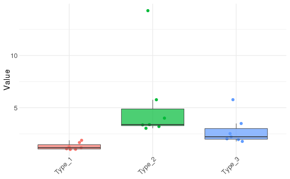
Sometimes I face problems in the lab for which I am not able to come up with a sensible answer, due to my lack of statistical knowledge. In this case, I have an answer, but I am not very sure if I am totally right, so I would like to describe my approximation and ask the community if it makes sense at all.
I am currently analyzing some gene expression data coming from an experiment on a set of cell lines.
The data (after being anonymized) looks like this:
|ID   |Type   |     Value|
|:----|:------|---------:|
|Id_1 |Type_1 |  1.064256|
|Id_2 |Type_1 |  1.000000|
|Id_3 |Type_1 |  1.016967|
|Id_4 |Type_1 |  1.249208|
|Id_5 |Type_1 |  1.659668|
|Id_6 |Type_1 |  1.876265|
|Id_7 |Type_1 |  1.169406|
|Id_1 |Type_2 |  3.030309|
|Id_2 |Type_2 |  4.001117|
|Id_3 |Type_2 |  3.383119|
|Id_4 |Type_2 | 14.293665|
|Id_5 |Type_2 |  3.359315|
|Id_6 |Type_2 |  5.760926|
|Id_7 |Type_2 |  3.197459|
|Id_1 |Type_3 |  2.517612|
|Id_2 |Type_3 |  1.943949|
|Id_3 |Type_3 |  2.211084|
|Id_4 |Type_3 |  1.772899|
|Id_5 |Type_3 |  5.767478|
|Id_6 |Type_3 |  3.487883|
|Id_7 |Type_3 |  2.019733|
The researcher is asking if there are any statistically significant differences between the three types. More precisely, she wants to know if there are differences between a) Type_2 and Type_1 and b) Type_3 and Type_1. This is a very simple experiment with Type_1 as a reference group.
It can also be considered that the measures are paired if we take the ID variable into account. But in this question I am going to ignore that for the sake of clarity.
I am using general linear models throughout the whole analysis, that comprises this and other questions. I have to admit that there is possibly a emotional bias involved, since this kind of models are quite intuitive for me. So, I proceed and fit a linear model to the previous data.
> fit = lm(Value ~ Type, data = foo)
> summary(fit)

Call:
lm(formula = Value ~ Type, data = foo)

Residuals:
    Min      1Q  Median      3Q     Max
-2.2591 -1.0443 -0.2908  0.3688  9.0042

Coefficients:
            Estimate Std. Error t value Pr(>|t|)
(Intercept)   1.2908     0.9453   1.365  0.18893
TypeType_2    3.9986     1.3369   2.991  0.00784 **
TypeType_3    1.5264     1.3369   1.142  0.26853
---
Signif. codes:  0 ‘***’ 0.001 ‘**’ 0.01 ‘*’ 0.05 ‘.’ 0.1 ‘ ’ 1

Residual standard error: 2.501 on 18 degrees of freedom
Multiple R-squared:  0.3361,    Adjusted R-squared:  0.2623
F-statistic: 4.556 on 2 and 18 DF,  p-value: 0.02506
By looking at the previous output, I told the researcher that there was a significant difference between the Type_2 and Type_1 groups, but not between the Type_3 and Type_1, despite the fact that graphically it seems that both Type_2 and Type_3 are different from the reference group.
The researcher did not like the result, as she was expecting both comparisons to be statistically significant. So she asked me to do some t-tests on the same data.
> t.test(Value ~ Type, data = foo, subset = foo$Type != 'Type_3')

    Welch Two Sample t-test

data:  Value by Type
t = -2.5849, df = 6.0849, p-value = 0.04097
alternative hypothesis: true difference in means is not equal to 0
95 percent confidence interval:
 -7.7709913 -0.2261915
sample estimates:
mean in group Type_1 mean in group Type_2
            1.290824             5.289416
Looking at the t-test result, we could say that there is a significant difference between Type_2 and Type_1. This is coherent with the linear model. What happens if we test the second hypothesis?
> t.test(Value ~ Type, data = foo, subset = foo$Type != 'Type_2')

    Welch Two Sample t-test

data:  Value by Type
t = -2.7643, df = 6.6979, p-value = 0.02919
alternative hypothesis: true difference in means is not equal to 0
95 percent confidence interval:
 -2.8441619 -0.2086578
sample estimates:
mean in group Type_1 mean in group Type_3
            1.290824             2.817234
Things are getting interesting. The result from this second t-test says that there is a significant difference between Type_3 and Type_1. Moreover, the p-value is smaller than the p-value for the first hypothesis. This is quite the contrary to what the results from the linear model are describing.
The researcher asked me if I could explain what was happening. I told her first that different methods can yield different results, especially when we are near the limit of statistical significance, and second, that the linear model approximation takes into account the variance of the whole dataset, even when it is testing a difference between two levels of a variable. I argued that the relationship between the variances (within and between groups) might be influencing the standard error computations and thus the final p-values.
With this in mind, I am wondering about a couple facts:
- Is the linear model approximation a good approach for this analysis or am I committing a terrible mistake?
- If the t-test or Wilcoxon (not shown, similar to the t-test) are generating positive results, why do we obtain such a high p-value (0.26853) for the corresponding coefficient in the linear model?
- Why such a penalization on the standard error for the Type_3 coefficient in the linear model when there is clearly much more variance in the Type_2 group?
Hope somebody can help me understand this to a greater extent. Any hint or help would be much appreciated.

