On the existence of a heavy-tailed c.d.f. given a condition based on the CLT

Question

My question is about the existence of a heavy-tailed distribution $F$ such that: given two i.i.d. samples $\{X_1,\ldots,X_n\}$ and $\{Y_1,\ldots,Y_n\}$, from $F$, we have

$$\sqrt{n}\frac{\hat{\mu}_X - \hat{\mu}_Y}{\hat{\sigma}}\rightarrow N(0,1)\text{ in distribution}$$

where $$\hat{\mu}_X=\frac{1}{n}\sum_{i=1}^nX_i,$$ $$\hat{\mu}_Y=\frac{1}{n}\sum_{i=1}^nY_i,$$ $$\hat{\sigma}^2 = \frac{1}{n} \left( \sum_{i=1}^n(X_i - \hat{\mu}_X)^2 + \sum_{i=1}^n(Y_i - \hat{\mu}_Y)^2\right).$$

Answer 1

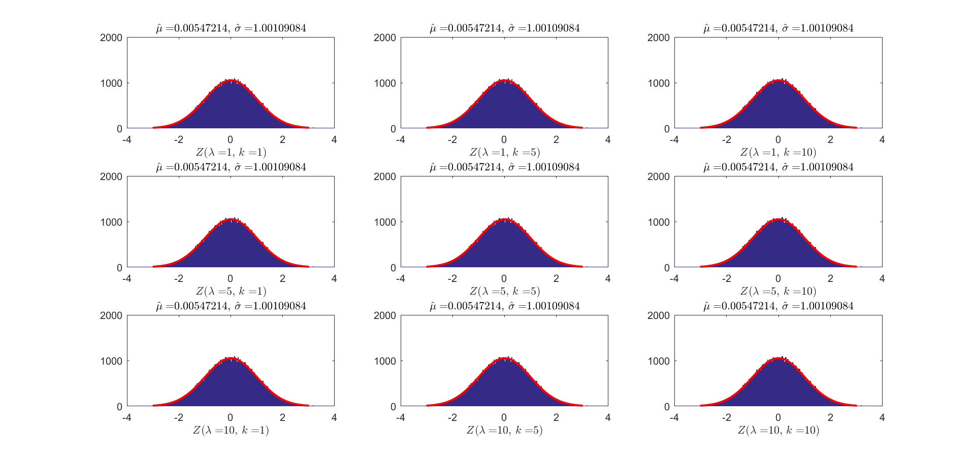
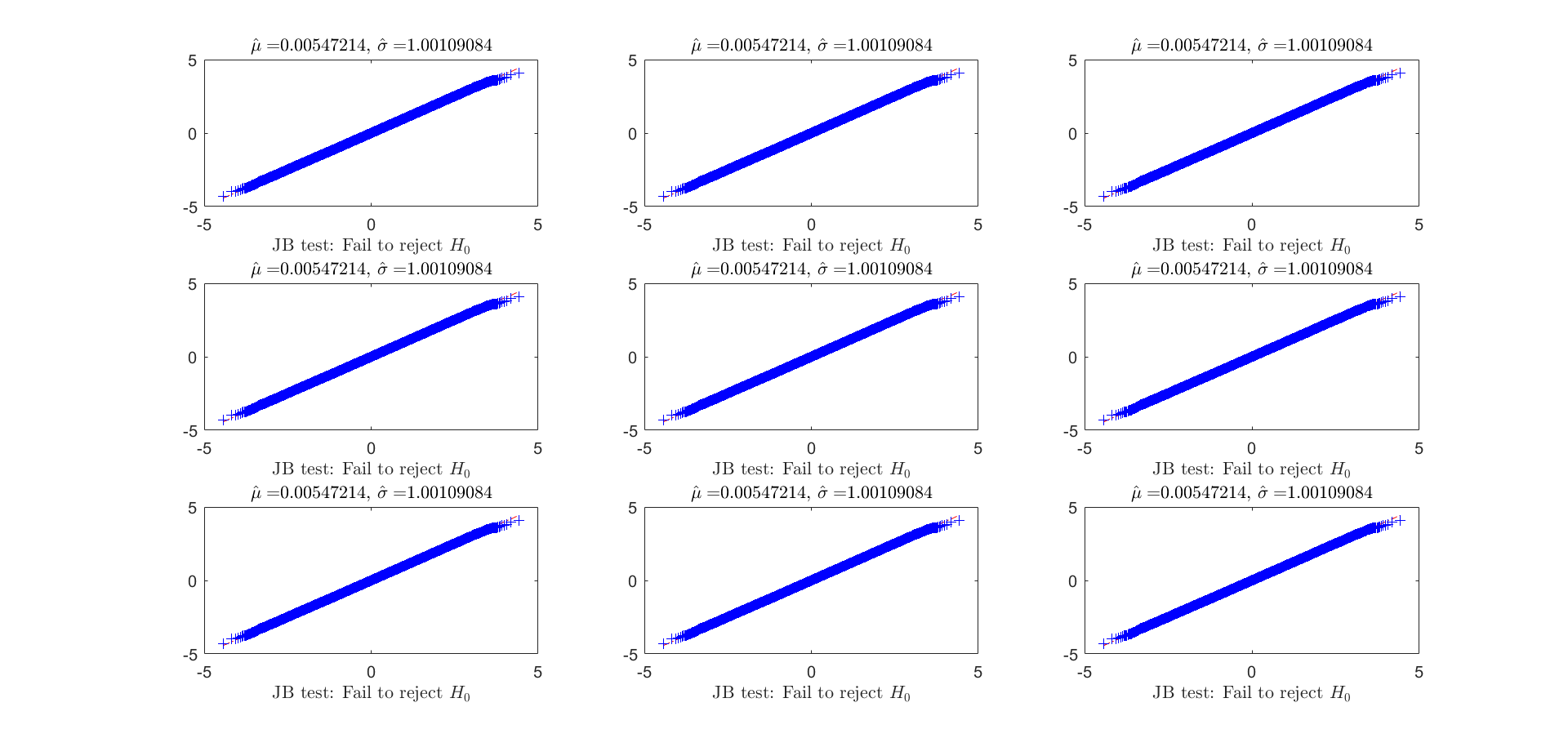
I can't prove the existence of a heavy-tailed distribution that will converge to a standard normal as you've described but I did some basic simulations that seem to suggest it could be the case.

Firstly, let's take the Weibull distribution, which is a heavy-tailed distribution. We'll define:

$$X,Y\sim W(\lambda,k)$$

where $\lambda$ and $k$ refer to the shape and scale of the Weibull distribution, respectively. Let's further assume $X$ and $Y$ to be independent. Now, if we define the following:

$$\hat{\mu}_{X}=\frac{1}{n}\sum_{i=1}^{n}X_{i}$$ $$\hat{\mu}_{Y}=\frac{1}{n}\sum_{i=1}^{n}Y_{i}$$ $$\hat{\sigma}^{2}=\frac{1}{n}\bigg(\sum_{i=1}^{n}\big(X_{i}-\hat{\mu}_{X}\big)^{2}+\sum_{i=1}^{n}\big(Y_{i}-\hat{\mu}_{Y}\big)^{2}\bigg)$$

You are looking for the following to be true:

$$Z=\sqrt{n}\bigg(\frac{\hat{\mu}_{X}-\hat{\mu}_{Y}}{\hat{\sigma}}\bigg)\overset{d}{\rightarrow} N(0,1)$$

Using the Weibull random variables defined above, I performed simulations by randomly sampling $n=10000$ times from each of $X$ and $Y$ and calculating the values defined above. I then repeated this process $m=100000$ times to test the convergence we postulated above.

The following plots show the distributions obtained for the simulations. I ran the simulation for 9 different $(\lambda,k)$ pairs to see if the behaviour changes as parameters of the Weibull change.

For each case, the MLE for the final distribution's parameters are calculated, assuming normality of the final distribution $(\hat{\mu},\hat{\sigma})$. As you can see, all the estimates for the mean and variance are close to what you are looking for. Furthermore, for each case, the Jarque-Bera normality test was applied to the sample which resulted in 9 failures to reject the null. I'll leave the interpretation of those results up to you.

I performed the simulations in MATLAB using the code below:

clear all
close all

n=10000;
m=100000;
p1=[1 5 10];
p2=[1 5 10];

figure(1)
figure(2)

for j=1:length(p1)
    for k=1:length(p2)
        for i=1:1:m
            s1=wblrnd(p1(j),p2(k),n,1);
            s2=wblrnd(p1(j),p2(k),n,1);

            mean1=mean(s1);
            mean2=mean(s2);
            std1=sum((s1-mean1).^2)/n;
            std2=sum((s2-mean2).^2)/n;

            a(i,1)=(mean1-mean2)/sqrt(std1+std2)*sqrt(n);
        end

        figure(1)
        set(gcf,'color','w')
        subplot(length(p1),length(p1),(j-1)*length(p1)+k)
        histfit(a)
        xlim([-5 5])
        m=mle(a,'distribution','normal');
        ttlstr=sprintf('$\\hat{\\mu}=$%.8f, $\\hat{\\sigma}=$%.8f',m(1),m(2));
        title(ttlstr,'interpreter','latex');
        parstr=sprintf('$Z(\\lambda=$%d, $k=$%d$)$',p1(j),p2(k));
        xlabel(parstr,'interpreter','latex');

        figure(2)
        set(gcf,'color','w')
        subplot(length(p1),length(p1),(j-1)*length(p1)+k)
        qqplot(a)
        m=mle(a,'distribution','normal');
        if jbtest(a)
            xlabel('JB test: Reject $H_{0}$','interpreter','latex');
        else
            xlabel('JB test: Fail to reject $H_{0}$','interpreter','latex');
        end
        ttlstr=sprintf('$\\hat{\\mu}=$%.8f, $\\hat{\\sigma}=$%.8f',m(1),m(2));
        title(ttlstr,'interpreter','latex');
        ylabel('');
        box on;
    end
end