Use the Fast Fourier Transform.
This post explains what that means, summarizes its advantages and limitations, presents the algorithm, analyzes its performance, illustrates it on data like that shown in the question, and gives working R code.
The distribution of the sum of random variables is the convolution of their distributions. Convolutions are most efficiently computed using the Fast Fourier Transform. The savings in time and memory are unlimited and can be enormous even in relatively small problems. This is faster and far more accurate then the other natural solution of estimating the distribution through simulation.
The price you pay is that the distributions must be discretized, as if they were "one-dimensional images." But since the FFT is so fast, you can discretize to a high precision--millions of bins ("pixels") are practicable, even though for many problems a hundred or a thousand bins will be more than enough resolution. (When you're willing to settle for such precision, Intel CPUs and various graphics coprocessors have native FFT implementations that will carry out the calculations with blazing speed.)
The principal limitation is that very skewed distributions, such as those with extreme outliers, could require an inordinate number of bins for a sufficiently precise computation. Such situations could be handled, if necessary, as mixture distributions: sum the mixture components, then mix the sums. In the interest of space I will ignore the details.
Here is the basic algorithm for finding the distribution of the sum of two empirical distributions for data $\mathbf{x}=(x_1, x_2, \ldots, x_m)$ and $\mathbf{y}=(y_1, y_2, \ldots, y_n)$. Its extension to more than two distributions is obvious (and illustrated in the code below); the only subtlety is that it's more efficient to apply the inverse FFT at the very end, rather than after each step.
Shift the data to make their minima both $0$. Afterwards, shift the result by adding the original minima back.
Choose the number of bins for the result. Divide the range of the result--which will go from $0$ to the sum of the (shifted) maxima--evenly into this number of bins. Classify each value in $\mathbf{x}$ into a bin, producing an array of counts indexed by the bins. Divide these counts by their total to produce a discretized frequency distribution. Do the same for $\mathbf{y}$.
Compute the FFTs of these arrays and multiply them componentwise.
At the end, take the inverse FFT of the result. Trim off any tiny imaginary components that might have crept in from floating point roundoff error. This is an array of relative frequencies of the sum for each of the bins defined in step (2).
The FFT algorithm scales by $(m+1)b\log(b) + n$ where there are $m$ input datasets with a total of $n$ values and you use $b$ bins. When $b\ll n$--which will be the case for any medium to large problem--this is a $O(n)$ algorithm. The brute-force algorithm is $O(n_1n_2\cdots n_m)$ where the individual datasets have $n_1, n_2, \ldots, n_m$ values. For instance, in the question $m=4$, $(n_1,n_2,n_3,n_4) = (4,10,2,8)$, $n=24$, and $n_1n_2n_3n_4=640$. It is obvious that this product rapidly grows much larger than the sum $n$.
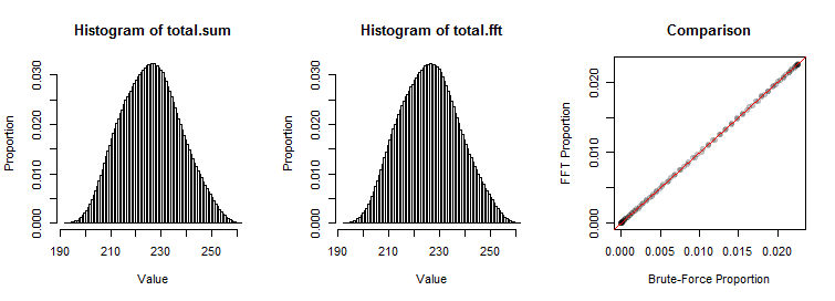
Here is an example comparing the two algorithms for an output of 6.4 million numbers. The brute-force method required a half second; the FFT method (with a thousand bins) took no measurable time.

The histograms, which use 100 bins, are indistinguishable. The "Comparison" at the right is a scatterplot of their values, showing the histograms are the same, bar for bar.
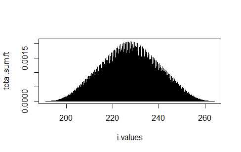
A similar problem with four input datasets, each one $10^4$ times greater, would require $(10^4)^4=10^{16}$ times as much computation and RAM for the brute-force method: that's out of the question. Timing for the FFT method (using 5000 bins for even greater precision) was a mere $0.17$ second. Most of that computation involved discretizing the input. Here is a barplot of its output:

This R code implements both algorithms. Their input is a list of arrays X. The output of the brute-force algorithm is total.sum. The output of the FFT algorithm is a pair of arrays: total.sum.ft contains the relative frequencies while i.values records the associated bin midpoints, as illustrated in the preceding graphic.
#
# Generate data.
#
factor <- 1e5
set.seed(12)
r.1 <- round(runif(n = 4*factor, min = 23, max = 50), digits = 1)
r.2 <- round(runif(n = 10*factor, min = 3, max = 15), digits = 1)
r.3 <- round(runif(n = 2*factor, min = 45, max = 49), digits = 1)
r.4 <- round(runif(n = 8*factor, min = 120, max = 150), digits = 1)
#
# Assemble and count them.
#
X <- list(r.1, r.2, r.3, r.4)
N <- prod(sapply(X, length))
message("There are ", N, " sums to compute.\n")
#
# Time the brute-force solution.
#
if (N < 1e8) {
  system.time({
    total <- expand.grid(X)
    total.sum <- rowSums(total)
  })
}
#
# Time the FFT solution.
#
system.time({
  #
  # Estimate the bin width.
  # `n.bins` is computed to (a) not be overly large
  # (excessive detail is rarely needed) and (b) to be larger
  # for larger datasets, which merit greater precision.
  #
  counts <- sapply(X, length)
  n.bins <- min(5e3, ceiling(100 * sqrt(max(counts))))
  range.sum <- rowSums(ranges <- sapply(X, range))
  dx <- diff(range.sum) / n.bins
  #
  # Initialize the FT of the sum.
  #
  x.hat <- rep(1, n.bins)
  #
  # Multiply the FTs of the components.
  #
  for (x in X) {
    #
    # Create a discrete representation of `x`.
    #
    i <- 1 + round((x - min(x)) / dx) # Compute the bins
    y <- tabulate(i, nbins=n.bins)    # Count the frequencies
    #
    # Accumulate the FT.
    #
    x.hat <- fft(y / sum(y)) * x.hat
  }
  #
  # Invert the FT of the sum.
  #
  total.sum.ft <- zapsmall(Re(fft(x.hat, inverse=TRUE))) / n.bins
  #
  # Compute the bin midpoints.
  #
  i.values <- (1:n.bins - 1/2) * dx + range.sum[1]
})
#
# Plot the two solutions.
# (`hist` cannot handle huge datasets.)
#
if (N < 1e8) {
  # -- Create a synthetic dataset consistent with the FFT representation,
  #    to be passed to `hist` for plotting.
  x <- round(N * total.sum.ft)
  total.fft <- unlist(mapply(function(i, n) runif(n, i-dx/2, i+dx/2), i.values, x))

  par(mfrow=c(1,3))
  # -- Set the histogram breaks
  B <- seq(range.sum[1], range.sum[2], length.out=101)
  # -- Plot two histograms
  h <- hist(total.sum, freq=FALSE, breaks=B,  xlab="Value", ylab="Proportion")
  h.fft <- hist(total.fft, freq=FALSE, breaks=B,  xlab="Value", ylab="Proportion")
  # -- Compare the histograms, bar by bar
  plot(h$counts/sum(h$counts), h.fft$counts/sum(h.fft$counts), pch=16, col="#00000040",
       main="Comparison",
       xlab="Brute-Force Proportion", ylab="FFT Proportion")
  abline(0:1, col="Red")
  par(mfrow=c(1,1))
} else {
  #
  # The datasets might be huge.  Settle for displaying the FFT solution.
  #
  plot(i.values, total.sum.ft, type="h")
}


