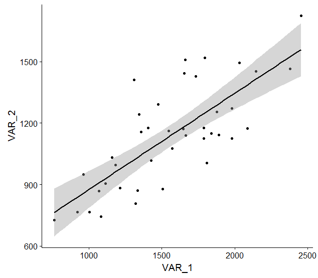
The following data frame df contains observations on two different measures of muscle strength (VAR_1 and VAR_2) from 24 males and 16 females. Both variables present a fairly linear relationship:
library("ggplot2")

ggplot(df, aes(x = VAR_1, y = VAR_2)) +
  geom_point() +
  geom_smooth(method = "lm", color = "black")
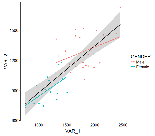
However, a closer look at GENDER reveals that Females are mainly locaten in the lower left part of the plot:
ggplot(df, aes(x = VAR_1, y = VAR_2)) +
  geom_point(aes(color = GENDER)) +
  geom_smooth(method = "lm", color = "black") +
  geom_smooth(aes(color = GENDER), method = "lm", se = FALSE)
The fact that females present lower outcomes in both variables affects modeling predictions including the entire dataset or only data from one gender. However, although women are usually weaker than men, there is no rationale to think that the relationship between both VAR_1 and VAR_2 is gender dependent.
Are there any "best practices" when it comes to fairly evaluating and interpreting the relationship between these two variables, accounting for any potential effect of GENDER?
Here we have some linear regressions including the entire data set:
fit <- lm(VAR_2 ~ VAR_1, data = df)
summary(fit)
Which results in:
> summary(fit)
Call:
lm(formula = VAR_2 ~ VAR_1, data = df)

Residuals:
    Min      1Q  Median      3Q     Max
-250.35 -114.86  -39.01  111.72  388.73

Coefficients:
             Estimate Std. Error t value Pr(>|t|)
(Intercept) 406.87642  104.55822   3.891 0.000389 ***
VAR_1         0.46927    0.06506   7.212 1.27e-08 ***
---
Signif. codes:  0 ‘***’ 0.001 ‘**’ 0.01 ‘*’ 0.05 ‘.’ 0.1 ‘ ’ 1

Residual standard error: 164.3 on 38 degrees of freedom
Multiple R-squared:  0.5779,    Adjusted R-squared:  0.5668
F-statistic: 52.02 on 1 and 38 DF,  p-value: 1.271e-08
Or accounting for GENDER in the linear regression call:
fit_gender <- lm(VAR_2 ~ VAR_1 + GENDER, data = df)
summary(fit_gender)
Which gives:
> summary(fit_gender)

Call:
lm(formula = VAR_2 ~ VAR_1 + GENDER, data = df)

Residuals:
    Min      1Q  Median      3Q     Max
-284.07 -113.23  -43.72  104.85  262.45

Coefficients:
               Estimate Std. Error t value Pr(>|t|)
(Intercept)   804.85032  176.94587   4.549 5.64e-05 ***
VAR_1           0.26776    0.09621   2.783  0.00843 **
GENDERFemale -210.73340   78.39083  -2.688  0.01070 *
---
Signif. codes:  0 ‘***’ 0.001 ‘**’ 0.01 ‘*’ 0.05 ‘.’ 0.1 ‘ ’ 1

Residual standard error: 152.3 on 37 degrees of freedom
Multiple R-squared:  0.6468,    Adjusted R-squared:  0.6278
F-statistic: 33.88 on 2 and 37 DF,  p-value: 4.339e-09
Data frame:
df <- structure(list(GENDER = structure(c(1L, 1L, 1L, 1L, 1L, 1L, 1L,
1L, 1L, 1L, 1L, 1L, 1L, 1L, 1L, 1L, 1L, 1L, 1L, 1L, 1L, 1L, 1L,
1L, 2L, 2L, 2L, 2L, 2L, 2L, 2L, 2L, 2L, 2L, 2L, 2L, 2L, 2L, 2L,
2L), .Label = c("Male", "Female"), class = "factor"), VAR_1 = c(2032.95602228266,
1645.84136319679, 1795.26082107151, 1547.11851437409, 1473.71473099518,
1654.41457933987, 2085.89855247696, 1840.30988797414, 1731.83124703822,
1892.49168271771, 1659.2423200817, 2379.84411458054, 1342.45455728821,
1309.87878136455, 1787.29982936431, 2147.67880389956, 1663.31028977522,
1982.42647407018, 1982.39817891865, 2454.85027809758, 1876.8911269728,
1788.31575689296, 1807.61528947627, 1571.47753963486, 962.514829411152,
1182.58776863074, 1424.9201681673, 1214.0785590926, 1334.2561628931,
1406.04081361931, 918.426537504858, 1321.03726255393, 1112.46568701098,
1082.76212547093, 1157.27133152872, 1003.82141604491, 761.377814135862,
1357.58749106345, 1067.86384075784, 1504.80678366675), VAR_2 = c(1495.11161840391,
1171.28580423435, 1517.91576982039, 1160.83516847309, 1290.3390955332,
1441.8949803003, 1174.30294841121, 1150.19303667107, 1427.70217475294,
1142.25248430695, 1510.12367036879, 1464.08394200785, 1243.4746868308,
1410.30146350545, 1175.79442393805, 1452.33610135076, 1139.05191957201,
1125.09462604151, 1271.39561360677, 1724.61669651112, 1255.6498053177,
1126.06937977549, 1004.78747531315, 1076.94960273115, 948.981977327285,
994.937522527885, 1016.5226800106, 883.513636610965, 871.08484388274,
1177.64099985273, 765.812857284995, 807.463314572285, 906.32646936372,
744.15494510974, 1031.9543118962, 764.79678843817, 725.83893532882,
1157.98504077507, 868.308441582335, 877.61788082039)), .Names = c("GENDER",
"VAR_1", "VAR_2"), row.names = c(NA, -40L), class = c("tbl_df",
"tbl", "data.frame"))


