What is a good way to measure the "linearity" of a dataset?

Question

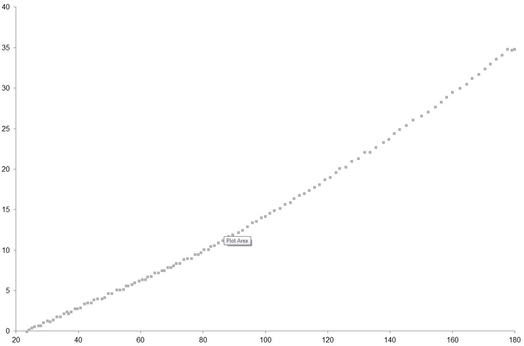
I have an empirically gathered dataset which relates two variables. Over a small range the relationship appears linear, however over a larger range there is clearly some second order polynomial relationship as can be seen in the image:

I'm trying to get a measure of linearity for different ranges considered. E.g. at 20 < x < 60 or 100 < x < 120 it is very linear, but at 20 < x < 180 it is not very linear. I have tried to fit a straight line to the data and calculate the R^2 data (goodness of fit) but this shows that the straight line over the larger range has a better fit than over the smaller range. While this may be true with MS Excel, from the image it is clear that the larger range is less linear...if you hold the side of a piece of paper against the points.

Is there a better way to measure the "linearity" of a dataset?

Answer 1

Fit a quadratic instead of a linear function. The absolute value of the estimate of the highest coefficient of the quadratic serves as a sensible measure of linearity, which is zero if the data lie exactly on a line. Moreover, if the data come from a linear model with Gaussian noise, the Gauss-Markov theorem guarantees that the coefficient estimates are unbiased, hence under repetition of the fit with multiple data from the same model distribution, the expected value of the coefficient will be zero.

Of course in a single fit, one usually doesn't get zero, so one would have to use some test for the significance of the coefficients.

Answer 2

One way to go would be to run a hierarchical regression with your Y-axis variable as the outcome/criterion. In step/block 1 you would enter your X variable as a predictor, and in step/block 2, enter a product term (X squared or multiplied against itself). The X squared term represents your quadratic component. The standardized regression weights (betas) for X and X squared would give you some sense of the "strength" of the linear and quadratic components relative to each other, and the change in R-squared from step/block 1 to step/block 2 is an indication of how much better the model fits the data when you have added in the quadratic component.

See Ch. 8 in Keith, T. Z. (2005). Multiple regression and beyond. Allyn & Bacon. 978-0205326440

Answer 3

The best measure of linearity between two variables x and y is the Pearson product moment correlation coefficient. The closer it is to 1 in absolute value the closer the fit is to a perfect straight line. Now if you think there is good linearity in a subregion, calculate the correlation for just those pairs in the subregion. If there is achange in shape outside that region it should show up in a drop in the correlation when all the data are included.

Answer 4

The standard statistical tools are the correlation coefficient (see Michael Chernick's answer) which is a value between [-1,1] and is unit independent. Related to the correlation coefficient is the covariance. The covariance is affected by units but may be easier to interpret. However, I don't like either of those options in the general case. I don't like them because they are not conformal transformation independent. Consider that a straight horizontal or vertical line is deemed to be non-linear by both of those measures.

A better unitless option is to use a singular value decomposition (SVD). The SVD breaks data up into component pieces ranked by magnitude of their contribution to the whole. The ratio of the largest singular number to the second largest singular number is hence a metric of linearity. Note, that to use this method you must first centralize the data (make average X, Y, Z, etc coordinates equal zero).

Example: Pts: 1126640.141 233575.2013; 1126630.008 233572.8567; 1126625.829 233572.7434;
1126625.416 233577.3781;

Centralized Pts: 9.792639127 0.656480018; -0.340591673 -1.68817349; -4.519928343 -1.801499913; -4.932119113 2.833193384;

SVD, D matrix: 11.86500017 0; 0 3.813448344

Ratio of singular Values 3.111357

The ratio above can be roughly interpreted as the data being three times as long in the direction of the best fit line as it is cross-linear.

For a solution with units that has units and doesn't require an SVD. Do some line fit that has the center of the line as one of the parameters. Using the centralized data above this is simple: line pt = 0 0 (always the case for centralized data) line direction = -0.999956849 -0.009289783

Vectors from the center of the line to each point are the centralized coordinates of the points. Find the lengths of the of the projection of these vectors onto the line (absolute value of the vector dot the line direction), and the length of the perpendicular vector component (length of vector cross line direction). Length Parallel, Length Perpendicular 9.798315123, 0.565480194; 0.356259742, 1.684936621; 4.536468847, 1.759433021; 4.905586534, 2.878889448;

The maximum of parallel projections is the stretch of data along the line. The maximum length of the perpendicular projection is a measure of the non-linearity. The ratio of the two is an approximation of the singular values ratio above.

Notes 1. Affine invariance in linearity is not possible. Consider, in an affine transformation we could scale all but one of the coordinate axes to near zero (making any set of points linear). So conformal invariance is the best we can do. 2. These methods are NOT ROBUST to outlier data. 3. Examples are 2D but generalized to N-dimensional.

Answer 5

I can't speak for the value of this approach, but this source suggests the following approach I'd not seen before (which I've rewritten into R code).

lin.tester.func <- function(x,y) {

  Sz.func <- function(z) {
    Sz1 <- sum(z^2)
    Sz2 <- sum(z)^2
    divZ <- Sz2 / length(z)
    Sz <- Sz1 - divZ 
    Sz
  }

  Sx <- Sz.func(x)
  Sy<- Sz.func(y)
  SsqrtXY <- sqrt(Sx) * sqrt(Sy)
  Sxy <- sum(x * y) - ((sum(x) * sum(y)) / mean(length(x),length(y)))
  Sxy / SsqrtXY
  # closer to 1, the more linear. 
}

• ^{Please edit if you know a name to this approach and please comment on utility/validity.}

Answer 6

One very simple way I have measured non-linearity before is based on the variation of the gradients between data points (using the difference in their x and y values). I then take the relative average deviation of the gradients, giving a value independent of the scale:

$$ Nonlinearity = RAD\bigg(\frac{diff(Y)}{diff(X)}\bigg) $$ Which is the same as doing $$ Z=\frac{diff(Y)}{diff(X)} \\ Nonlinearity=\frac{MAD(Z)}{mean(Z)} $$

where Y and X are the vectors from the pairs of values. diff() means the difference between one value and the previous (i.e. x[n+1]-x[n]). mad() is mean absolute deviation.

This measures non-linearity because any two points on a line have the same gradient between them, therefore the mad() or std() of the gradients between points will be zero if the points are on a line, and larger the more the gradients deviate. I created this measure independently, so it may already be described with an actual name or there may be a similar but better approach, but it's intuitive and simple.

You can also use std dev instead of RAD, which results in taking the coefficient of variation of the gradients, cv():

$$ Nonlinearity = cv\bigg(\frac{diff(Y)}{diff(X)}\bigg) $$

Measures like CV, SD and correlation coefficient weigh outliers more heavily, so under some circumstances you may prefer RAD, which gives a more linear measure of non-linearity. You can also calculate the ratio of RAD to CV, which gives further information about your data.

Either of these can easily be adapted to give a measure of linearity between 0 and 1:

$$ Linearity = \frac{1}{1+\frac{MAD(Z)}{mean(Z)}} $$

or

$$ Linearity = \frac{1}{1+cv(Z)} $$