Are predictive distributions supposed to be distributions of future data?

Question

In frequentist analysis, we define a 95% prediction interval as an interval that will contain the next observation 95% of the time under repeated sampling of the entire experiment and prediction. If we are dealing with a scalar observable, we may even be able to turn this into a type of "predictive distribution" (in the Fiducial sense).

This all makes sense to me, since the interval and/or distribution are not purporting to be the actual distribution of the next point, only devices for making predictions with the correct operating characteristics.

In contrast, I've just finished reading Gelman et al's Bayesian Data Analysis (3rd ed) and I have an issue with how to interpret the posterior predictive intervals that are calculated for posterior predictive checks. In Dr. Gelman's view, our prior + likelihood both constitute our stochastic model of the data generating process. In this model, "nature" first draws a value for the true parameter, then generates observations using this parameter. Note: For the rest of my quesion, please remember that the Bayesian model assumes nature did this only once, to fix our parameter, and then started generating values.

Now, let's say we want to compare our fitted model by comparing the distribution of our model to the actual values from our experiment (say, of size 100). To do this, Gelman suggests we simply generate $M$ draws from the posterior distribution of the parameters and then, for each draw, draw a sample of 100 values from the associated data model (likelihood). This is essentially assuming that each sample of 100 observations gets its own (different) parameter from the posterior distribution; therefore, the resulting distribution will generally be wider than if we simulated future values using the known (true) parameter value that actually generated the data.

And here's where I have in issue: Let's say I plan to take 10,000 more observations from the same process (i.e., predict what I would have seen if I had extended the experiment beyond 100 observations). In this case, it's provably true that these 10,000 observations will not follow the posterior predictive distribution, since the posterior predictive distribution includes variability/randomness in the underlying parameter, but the actual data are being generated from a fixed parameter (see my note from above). Hence, posterior predictive distributions do not give an accurate picture of the distribution of future observations.

So, if this is the case, how can comparing the observed data (which does not actually have parameter variability) with the fitted posterior predictive distribution help us except to see gross errors? Even if our Bayesian model were 100% correct, the posterior predictive distribution would still be wider than the true data distribution.

Can someone explain what a posterior predictive distribution is actually modeling?

---

Aside

Perhaps I'm interpreting the posterior predictive distribution too literally (but I could be forgiven given it's use by Gelman). Maybe the "posterior predictive distribution" is simply a measure over the range of the observations that allows you to assign a probability to an interval. It implies that since we don't know the true value of the parameter, we are averaging over all possible models in proportion to their posterior probability.

In this way, posterior predictive distributions are closer to a mixture distribution, than to the true distribution of the data: the distribution "averages over" possible futures, but will not necessarily reflect any particular future (a large sample of new observations will not look like the posterior predictive distribution).

This has a repeated sampling interpretation: if we repeatedly drew new experiments from our Bayesian model, conditional on getting the exact same observations we actually did, then took an additional 1000 observations each time, a 90% posterior prediction interval will contain approximately 90% of these observations on average. This is just like frequentist prediction intervals.

Answer 1

You almost wholly and correctly answered your blog question. I created a few simulations to show you where the differences are.

Also, I have a personal issue with the term of art, “overdispersed.” Predictive distributions are not overdispersed, they are correctly dispersed, but the true distribution in nature doesn’t match it. Instead, it is contained within it.

The two types of predictions differ in a number of subtle ways. Which type of prediction to use should depend wholly on the actual problem you face and the losses you face from unfortunate sampling or other issues.

The first difference comes from the existence of prior information. In the absence of prior information, Frequentist methods minimize the maximum possible loss you could face from a bad estimator. That is very advantageous when you have no framework to estimate an average loss instead. Bayesian methods minimize the average loss experienced, but the prior does matter. In the presence of prior information, all Frequentist solutions are inadmissible. Furthermore, Frequentist methods do not give rise to coherent probabilities and so should never be used in gambling situations such as estimating inventory needs, portfolio allocations or budgets.

The question of whether you should use a Bayesian density or a Frequentist interval should depend only on the problem you are solving.

I decided to exaggerate your example a little by expanding a metaphor I use a lot to teach the differences in prediction methods. I modified the game as well to fit the Reverand Bayes original example because it had both a Bayesian and a strong Frequentist interpretation. Although the Reverand Bayes used a billiards table to generate a uniformly distributed random number, I used the R language function runif().

Using seed 9817, I drew a value of the parameter of 0.5171191. Based on this parameter value eight Bernoulli trials were performed. There were four successes. The question is now to predict the number of successes, based on the eight observed trials, over the next 10,000 observations. Knowing the conditions of the generation of the parameter, I used a uniform prior density for the Bayesian solution.

The Frequentist solution is an interval, but it does generate a density from which to create an interval. For a binomial likelihood, the Frequentist prediction interval is constructed from the hypergeometric distribution. For the Bayesian method, the prediction is a one-dimensional Polya distribution. They are very close, but they are importantly different.

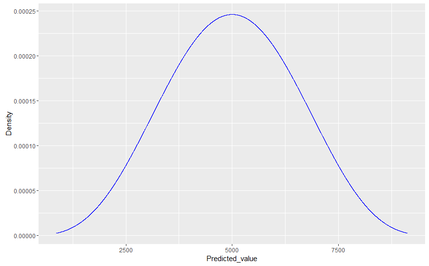
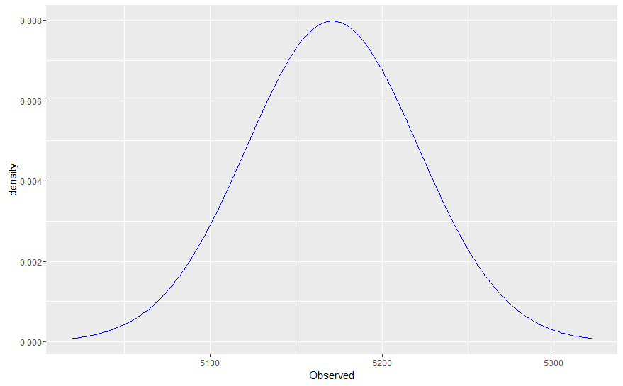
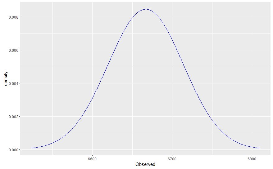
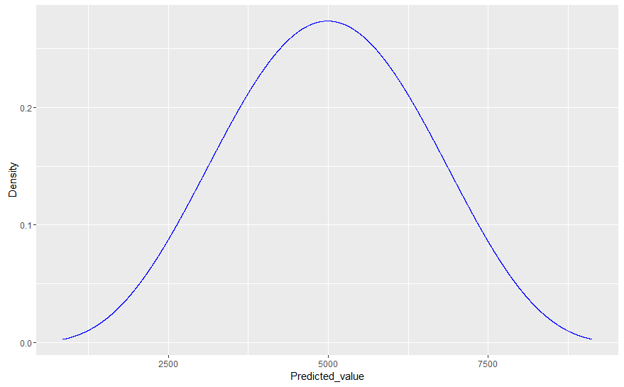
The Frequentist density from which to construct intervals is shown here, while the Bayesian density is shown here, if the true value of the parameter were known, then the prediction would be this one instead.

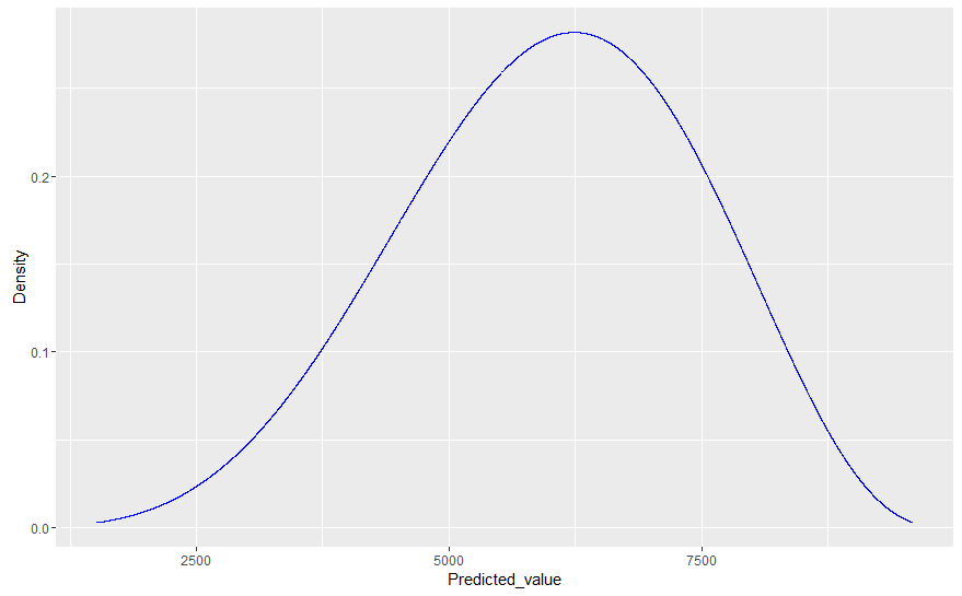
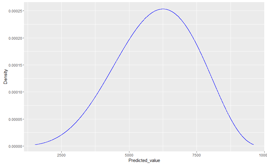
To get a better feel, also consider the cases where the true value were 2/3, and there were five successes in eight trials. The Frequentist is,

the Bayesian is,

the true prediction is.

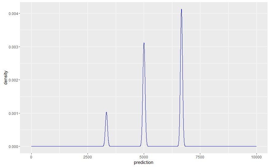
Now as to the differences, imagine that the parameter space was discrete. Let us consider the case where the only three possibilities were a parameter space of $\{1/3,1/2,2/3\}.$ There isn’t a known way to construct predictive intervals on discrete parameter spaces. If the prior were uniform, then the Bayesian predictive distribution would be like this.

Of course, this is not the only difference. There is only one way to construct a Bayesian predictive density, but there is an infinite number of predictive intervals because predictive intervals are built on top of confidence intervals. They depend entirely on the cost function chosen. As such, the Frequentist interval that is usually taught as “the” Frequentist interval is the one that minimizes the average loss under the Kullback-Leibler Divergence. It is not uniquely the Frequentist prediction interval method. Change the loss function, and you will change the boundaries.

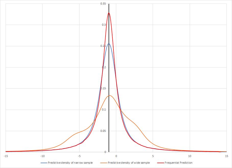
The reason this is usually used is that the Bayesian predictive density automatically minimizes the Kullback-Leibler Divergence. Note I did not say it minimized the average divergence, but the actual divergence. To illustrate the differences, I drew two samples from $$\frac{1}{\pi}\frac{1}{1+(x-\mu)^2}.$$ The samples were $\{-1.5,-1,-.5\}$ and $\{-6,-1,3\}.$ Because there are issues with using the maximum likelihood estimator on small samples from this distribution, I used the median instead. At this sample size, the information loss is trivial for the accuracy gained. One of the nice things about the Frequentist interval method is that it can be created from any statistic with a sampling distribution, although if you change the statistic, then you change the predictions. As it is known there is no analytic solution to the above problem, I created the prediction by drawing 10,000,000 samples of size four. I used the first three observations to create the statistic, and the fourth was to be predicted.

Note that because both samples share the same median and because both samples have the same known scale parameter, the distribution from which to construct the Frequentist prediction intervals is the same for both. It is an averaging process — the Frequentist method controls for worst-case samples. It minimizes average loss, but not a specific loss as the Bayesian method would.

There are a few other minor differences. A Frequentist prediction interval is uniformly distributed over the interval. There are no dense areas. Its interpretation would be that upon repetition, and $\alpha$ percent prediction interval will cover the prediction no less than $\alpha$ percent of the time.

A Bayesian interval would be interpreted as having an $\alpha$ percent probability of containing the future sample. Of course, for both, it is contingent upon the prior sample actually seen. Furthermore, there is an infinite number of intervals from a Bayesian density because there is no restriction that you use the highest density region. You could choose the lowest density region if you wished. Any subset of the density that adds to $\alpha$ percent is a valid $\alpha$ prediction interval. The highest density region is usually used because it has other optimality properties.