Simulate CDF of sum of i.i.d. F distributions

Question

I have trouble on simulating the CDF of a random variable Y, where $Y = \sum_{i=1}^{12} X_i$, and $X_i$ are i.i.d. F-distribution.

I am doing this in MATLAB, the problem is that small instance of Y hardly occurs. I don't think I can use Importance Sampling since I don't know the density function of Y(I doubt there is an analytic formula). Central Limit Theorem won't work since 12 isn't very large.

What should I do? Thanks!

Answer 1

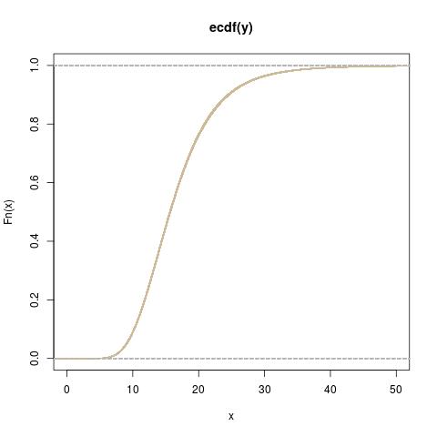
I am not certain what you mean by "simulating the cdf of Y". From a simulated sample of $Y$'s you can certainly plot the empirical cdf. For instance,

y=apply(matrix(rf(12*1e5,df1=3,df2=7),ncol=12),1,sum)
plot(ecdf(y))

returns an empirical cdf in R. The precision of this approximation is provided by the Binomial nature of the empirical cdf, namely$$N\hat{F}(x)\sim\mathcal{B}(N,F(x))$$To show this precision I plotted 100 independent realisations of the above code on the same graph: the variability is of the order of the thickness of the lines used to draw the cdf.

The issue of not getting samples of $Y$ close to zero is an altogether different question that you should rephrase with more details.

However, one generic remark about the density of $Y$ being unavailable for basic importance sampling is that one can use Monte Carlo (de)marginalisation to get around the issue. Given that the density of $(X_1,\ldots,X_{12})$ is available as $$\prod_{i=1}^{12} \mathfrak{f}(x_i|\nu_1,\nu_2)$$it suffices to choose an importance function (density) on $(X_1,\ldots,X_{12})$ that produces small values of $(X_1,\ldots,X_{12})$, $$\prod_{i=1}^{12} \mathfrak{g}(x_i)$$ and to use the importance ratio $$\prod_{i=1}^{12} \mathfrak{f}(x_i|\nu_1,\nu_2)/\mathfrak{g}(x_i)$$