How to estimate the Poisson distribution with one event occurrence?

Question

Let us say we observed one event on 1 Jan 2005, and we were observing the events since 2000. What's the best estimate of Poisson distribution?

One approach is to set intensity $\lambda=1/18$ per year. This is a Poisson MLE estimate, since we had 18 years passed and only one event observed.

Another approach seems to be fitting exponential distribution to time to arrival. Will they lead to the same estimate?

UPDATE

In my problem the estimation of Poisson intensity is conditional on the observation of a single event. This is an important factor, because it's not obvious that it doesn't mess up the usual MLE for Poisson.

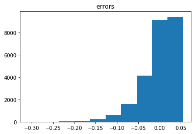
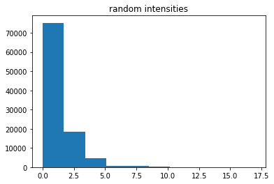
I ran a simulation where random intensities are drawn, then random frequencies are drawn from these intensities. We look only at frequencies equal to one in 18 years. Finally, we use intensity estimator that is equal to observed frequency, like in a usual MLE for Poisson, and compare to the true intensity.

I suspected that for rare events when event was observed precisely once in a sample period, there could be a better estimator of the Poisson intensity than the observed frequency. However, this simulation shows zero bias of the usual Poisson MLE.

import numpy as np
import matplotlib.pyplot as plt
import scipy.stats as stats

ns = 100000
T = 10
lam = np.random.gamma(1,1/T,ns) # random intensities ~1/18 (per year)
obsf = np.random.poisson(lam*T,ns) # observe frequencies for 18 years

plt.hist(obsf)
plt.title('random intensities')
plt.show()

sidx = np.where(obsf==1)[0] # we only look at trials where 1 event happened in 18 years
err = (obsf[sidx]/T - lam[sidx]) # error when intensity estimator is set to observed frequency
print(stats.describe(err))

plt.hist(err)
plt.title('errors')
plt.show()

output:

DescribeResult(nobs=25146, minmax=(-0.30917753984994045, 0.055486021558327742), mean=-0.00044121203771743959, variance=0.0015661042110224508, skewness=-1.434031238643681, kurtosis=2.993433694497429)

UPDATE 2

I used Gamma as the simulated parameter distribution. It's unfair, because Gama is a prior to Poisson. I'll use some other distribution.

Answer 1

I would treat this as one observation of, assuming you started at midnight on Dec. 31, 2000, 4 years, and another observation censored at 12.956 years. In the case of the exponential distribution, this is a pretty easy problem to solve:

$$p(x_1, x_2 | \lambda) = \left(\frac{1}{\lambda}e^{-x_1/\lambda}\right)\left(e^{-c_2/\lambda}\right)$$

where the first term is the probability of observing $x_1$ and the second the probability of observing $x_2 > c_2$, with $c_2$ being the censoring point of 12.956 years. Taking the log and setting the derivative equal to zero gives us:

$$\hat{\lambda} = \frac{1}{x_1 + c_2}$$

which gives us roughly $1/18$ years, as we are at the end of 2017 instead of the beginning.

This is just working through a specific case of the general result that the MLE for a censored Exponential distribution is equal to the sum of the total observed times, regardless of whether they were censored, divided by the total number of observed arrivals.

The conclusion: the two approaches will give the same result.

Edit in response to comments:

The Poisson and Exponential-based estimators will always give the same answer. In the case of the Poisson, you have $n$ events observed over the time period $T$ giving an estimate of $T/n$. In the case of the Exponential, your total observed time is $T$, and you have $n+1$ observations, with the last one being censored by the end of the observation period, so the estimate is $n/T$.

Answer 2

Looking more closely at your simulation, I can see a bit more clearly what you're doing. You've set up a data generating process with a random intensity taking a gamma distribution for each gamma intensity, there's a Poisson realization, you then turn to estimate the Poisson rate among a subsample with non-zero counts.

This is a bit different than how I envisioned the date problem because you have data from a sample, some of which are deliberately excluded, and this sample has important heterogeneity.

There's a couple things to address here: If you did not have a random input to the Poisson process, the correct probability model for the observed data is a zero-truncated Poisson distribution. https://en.wikipedia.org/wiki/Zero-truncated_Poisson_distribution. Note that a method of moments estimator for the intensity could be solved numerically (no tractable analytic solution)

\begin{equation} 0 = \bar{Y} - \lambda \exp(\lambda) / (\exp(\lambda) - 1) \end{equation}

set.seed(123)
ns <- 10000
zcpois <- function(y) uniroot(function(x) mean(y) - x*exp(x)/(exp(x)-1), c(1e-8, max(y)))
y <- rpois(ns, 0.7)
zcpois(y[y!=0]) ## very precise MoM

> zcpois(y[y!=0])$root
[1] 0.6950045

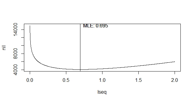
You can also use maximum likelihood recalling the likelihood for a truncated RV: $P(Y=y | Y>0) = P(Y=y)/P(Y>0)$.

y0 <- y[y!=0]
negloglik <- function(lambda, y) {
  -sum(dpois(x=y, lambda=lambda, log=T) - ppois(q=0, lambda=lambda, lower.tail=F, log=T))
}

lseq <- seq(from=0.001, to=2, by=0.001)
nll <- sapply(lseq, negloglik, y=y0)
plot(lseq, nll, type='l')
i <- which.min(nll)
abline(v=lseq[i])
text(lseq[i], max(nll), paste('MLE:', lseq[i]), pos=4, xpd=T)

However, it's important to consider the Poisson/Gamma mixture and the impact on the resulting probability model. The mixture model does not follow a zero-truncated Poisson distribution. The underlying Poisson process (without omission of 0 counts) would follow an overdispersed Poisson process.

lambdas <- rgamma(ns, 1, 18) ## rate parametrization
counts <- rpois(ns, lambdas)
nzcounts <- counts[counts!=0]

> zcpois(nzcounts)$root
[1] 0.1311875
> mean(lambdas)
[1] 0.05573894

A Bayesian model whose likelihood follows a zero-truncated Poisson model and whose intensity follows a gamma distribution with a non-informative shape and scale parameter would enable you to estimate the posterior distribution, whose posterior modes would give you good estimates of the input parameters to the gamma distribution. A frequentist approach would invoke the EM algorithm.