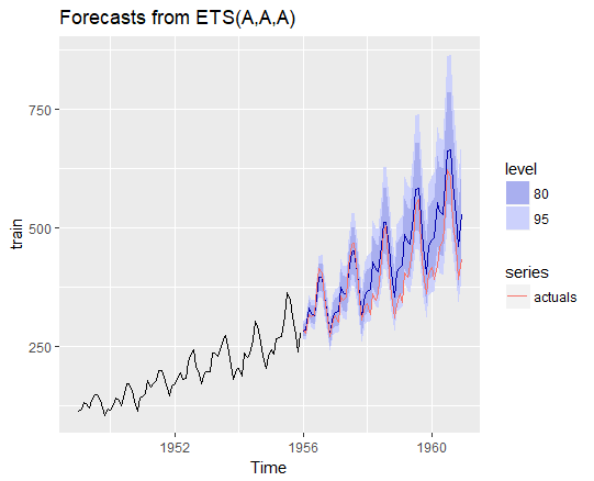
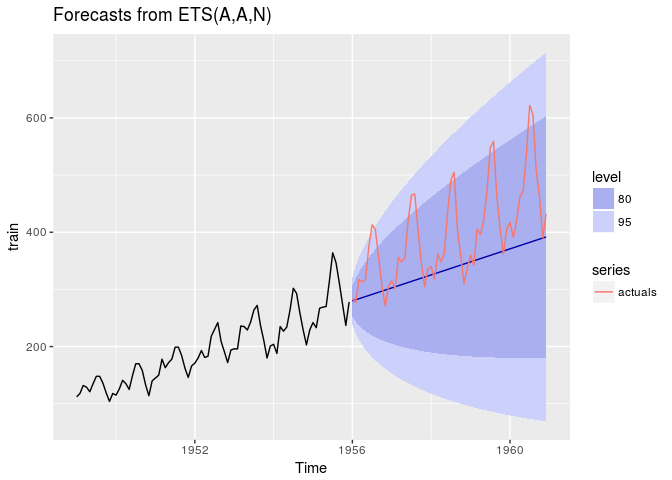
This is easily done using the general structure you've provided. Unfortunately, you left out the annual seasonal term, and consequently the algorithm was unable to estimate the seasonal component that contains most of the time series structure.
Note also that for this data the series seems to increase in a nonlinear fashion, as does the variability due to seasonal swings. This indicates that a Box-Cox transform may help.
The following code does what you want, with a little extra added for the Box-Cox transform. The confidence intervals, as plotted, do not contain the additional variability due to the estimation of the Box-Cox parameter $\lambda$, which, as it happens, equals $0$ - i.e., a log transform performed best according to a minimum AIC criterion.
library(forecast)
library(ggplot2)

train   <- subset(AirPassengers, end = 84)
actuals <- subset(AirPassengers, start = 85)

aic <- ets(train, "ZZZ", lambda=0, biasadj=TRUE)$aic
min_lambda <- 0
for (lambda in seq(0.05, 1, by=0.05)) {
   m2 <- ets(train, "ZZZ", lambda=lambda, biasadj=TRUE)
   if (m2$aic < aic) {
      aic <- m2$aic
      min_lambda <- lambda
   }
}
m2 <- ets(train, "ZZZ", lambda=min_lambda, biasadj=TRUE)
fc2 <- forecast(m2, h=60)
fc2 %>% autoplot() + autolayer(actuals)
which leads to the following graph:

Clearly this is not a very good forecast at the longer horizons, but in real life we'd probably forecast over a shorter horizon to start with and use out-of-sample predictions to select $\lambda$. In any case, the objective is to show you how to capture the annual structure and the confidence intervals of the forecasts in the model.
Now, on to something more like the question you really asked! The forecast object fc2 contains, as a default, 80% prediction intervals and 95% prediction intervals in the first and second columns respectively of fc2$lower and fc2$upper. We can extract these intervals from the forecast object as follows:
> ci <- data.frame(cbind(lower_95=fc2$lower[,2], upper_95=fc2$upper[,2]))
> head(ci)
         lower_95 upper_95
Jan 1956 263.7051 301.8168
Feb 1956 264.3147 307.9777
Mar 1956 302.9796 358.7300
Apr 1956 290.3735 348.8713
May 1956 285.0566 347.1562
Jun 1956 319.1490 393.6367
These are pointwise prediction intervals, in the sense that for each period taken individually there is an $\alpha$% probability of falling outside the interval (given all the assumptions.) However, forecast errors are autocorrelated, so the probability of falling outside the interval in, say, Feb. 1956 is not independent of whether or not we fell outside the interval in Jan. 1956; consequently, a t-test based on the errors over the whole forecast horizon would be biased due to the failure of independence.
Since forecast errors tend to be positively correlated for forecast models that take into account short-term dependencies in the variate of interest, we can apply Hochberg's step-up procedure (see here) for a joint test.
ci <- data.frame(cbind(obsno=1:60, lower_95=fc2$lower[,2], upper_95=fc2$upper[,2]))
ci$p_value <- 1-pnorm(abs((actuals-fc2$mean))/((ci$upper-ci$lower)/(2*1.96)))
ci <- ci[order(ci$p_value),]
ci$hochberg_cutoff <- 0.05/(61-1:60)
with result:
> head(ci)
   obsno lower_95 upper_95    p_value  hochberg_cutoff
51    51 421.3037 713.9750 0.03590013     0.0008333333
38    38 332.3203 525.6013 0.05502230     0.0008474576
28    28 336.5221 500.7919 0.06149721     0.0008620690
27    27 349.7245 517.0156 0.06288973     0.0008771930
36    36 323.5269 505.8235 0.06568278     0.0008928571
26    26 303.6777 445.9398 0.07688071     0.0009090909
which in this instance would not reject any time period as having fallen outside the Hochberg-corrected 95% test interval, as the minimum observed p-value is $>$ the Hochberg cutoff level.
There are plenty of other multiple comparison corrections, see for example the Wikipedia page, that may be more or less useful to you.


