Here is an example of estimating a mean, $\theta$, from Normal continuous data. Before delving directly into an example, though, I'd like to review some of the math for Normal-Normal Bayesian data models.
Consider a random sample of n continuous values denoted by $y_1, ..., y_n$. Here the vector $y = (y_1, ..., y_n)^T$ represents the data gathered. The probability model for Normal data with known variance and independent and identically distributed (i.i.d.) samples is
$$
y_1, ..., y_n | \theta \sim N(\theta, \sigma^2)
$$
Or as more typically written by Bayesian,
$$
y_1, ..., y_n | \theta \sim N(\theta, \tau)
$$
where $\tau = 1 / \sigma^2$; $\tau$ is known as the precision
With this notation, the density for $y_i$ is then
$$
f(y_i | \theta, \tau) = \sqrt(\frac{\tau}{2 \pi}) \times exp\left( -\tau (y_i - \theta)^2 / 2 \right)
$$
Classical statistics (i.e. maximum likelihood) gives us an estimate of $\hat{\theta} = \bar{y}$
In a Bayesian perspective, we append maximum likelihood with prior information. A choice of priors for this Normal data model is another Normal distribution for $\theta$. The Normal distribution is conjugate to the Normal distribution.
$$
\theta \sim N(a,1/b)
$$
The posterior distribution we obtain from this Normal-Normal (after a lot of algebra) data model is another Normal distribution.
$$
\theta | y \sim N(\frac{b}{b + n\tau} a + \frac{n \tau}{b + n \tau} \bar{y}, \frac{1}{b + n\tau})
$$
The posterior precision is $b + n\tau$ and mean is a weighted mean between $a$ and $\bar{y}$, $\frac{b}{b + n\tau} a + \frac{n \tau}{b + n \tau} \bar{y}$.
The usefulness of this Bayesian methodology comes from the fact that you obtain a distribution of $\theta | y$ rather than just an estimate since $\theta$ is viewed as a random variable rather than a fixed (unknown) value. In addition, your estimate of $\theta$ in this model is a weighted average between the empirical mean and prior information.
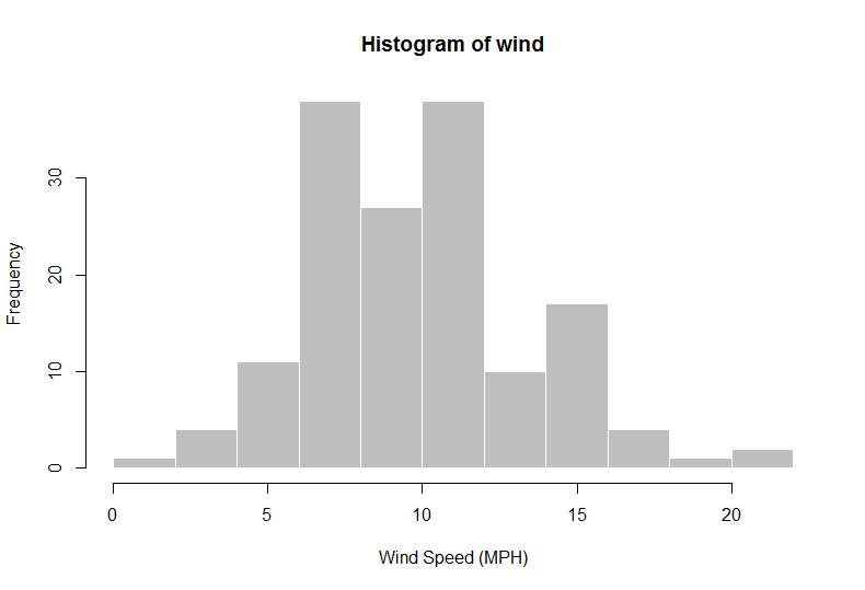
That said, you can now use any Normal-data textbook example to illustrate this. I'll use the data set airquality within R. Consider the problem of estimating average wind speeds (MPH).
> ## New York Air Quality Measurements
>
> help("airquality")
>
> ## Estimating average wind speeds
>
> wind = airquality$Wind
> hist(wind, col = "gray", border = "white", xlab = "Wind Speed (MPH)")
>

> n = length(wind)
> ybar = mean(wind)
> ybar
[1] 9.957516 ## "frequentist" estimate
> tau = 1/sd(wind)
>
>
> ## but based on some research, you felt avgerage wind speeds were closer to 12 mph
> ## but probably no greater than 15,
> ## then a potential prior would be N(12, 2)
>
> a = 12
> b = 2
>
> ## Your posterior would be N((1/))
>
> postmean = 1/(1 + n*tau) * a + n*tau/(1 + n*tau) * ybar
> postsd = 1/(1 + n*tau)
>
> set.seed(123)
> posterior_sample = rnorm(n = 10000, mean = postmean, sd = postsd)
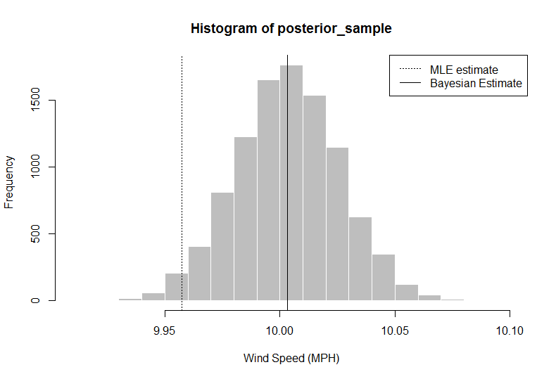
> hist(posterior_sample, col = "gray", border = "white", xlab = "Wind Speed (MPH)")
> abline(v = median(posterior_sample))
> abline(v = ybar, lty = 3)
>

> median(posterior_sample)
[1] 10.00324
> quantile(x = posterior_sample, probs = c(0.025, 0.975)) ## confidence intervals
2.5%     97.5%
9.958984 10.047404
In this analysis, the researcher (you) can say that given data + prior information, your estimate of average wind, using the 50th percentile, speeds should be 10.00324, greater than simply using the average from the data. You also obtain a full distribution, from which you can extract a 95% credible interval using the 2.5 and 97.5 quantiles.
Below I include two references, I highly recommend reading Casella's short paper. It's specifically aimed at empirical Bayes methods, but explains the general Bayesian methodology for Normal models.
References:
Casella, G. (1985). An Introduction to Empirical Bayes Data Analysis. The American Statistician, 39(2), 83-87.
Gelman, A. (2004). Bayesian data analysis (2nd ed., Texts in statistical science). Boca Raton, Fla.: Chapman & Hall/CRC.


