Strong linear pattern in residuals of random intercept model (simulated unbalanced data)

Question

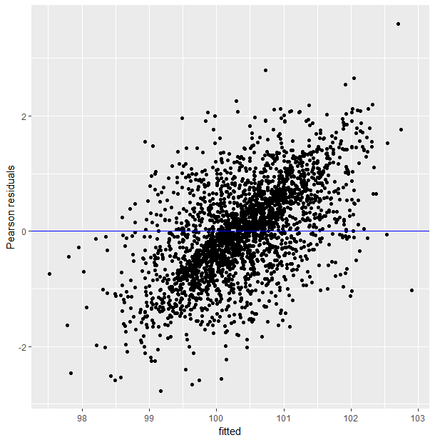
I am working with an unbalanced data set where most subjects have only 1 observation, but many have >1. When I fit a linear mixed model to these data (random intercept), there is a strong pattern in the residuals vs. fitted. I was able to duplicate the problem with simulated data (below).

The linear pattern seems to mostly come from individuals with only 1 observation.

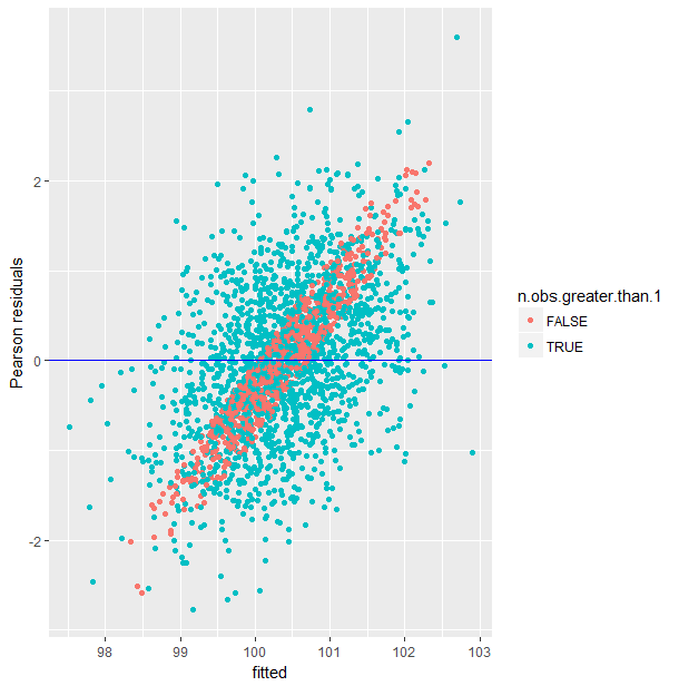
This is because the random effect estimate (i.e., ranef(model))for those individuals with only 1 observation is approximately equal to their residual (i.e., resid(model)).

So my question is, how do I assess the model fit for this mixed effects random intercept model via residual diagnostics given these type of unbalanced data?

Example data:

I borrowed the code below to simulate data from here.

This code block generates a balanced dataset with varying intercepts and 1 explanatory covariate. In the next block, I sub-sample this to create an unbalanced dataset, fit the model, and plot residuals vs. fitted.

#This code allows for random inercepts too, but I just set these parameters close to 0. 
library(lme4) 
form<-as.formula(c("~env+(env|ID)"))
N.ind<-2000
N.obs<-5
simdat <-data.frame(ID=factor(rep(1:N.ind,each=N.obs)),env=runif(N.ind*N.obs,0,1))
beta<-c(100,0.8)
names(beta)<-c("(Intercept)","env")

V.ind0 <- 1
V.inde <- 0.01
V.err0 <- 1
COVind0.ind1e <- 0.01*(sqrt(V.ind0*V.inde))

vcov<-matrix(c(V.ind0,COVind0.ind1e,COVind0.ind1e,V.inde), 2, 2)

theta<-c((chol(vcov)/sqrt(V.err0))[1,1],
         (chol(vcov)/sqrt(V.err0))[1,2],
         (chol(vcov)/sqrt(V.err0))[2,2])
names(theta)<-c("ID.(Intercept)","ID.env.(Intercept)","ID.env")

#set.seed(25)
response<-simulate(form,newdata=simdat,family=gaussian,
                   newparams=list(theta = theta,beta = beta, sigma = sqrt(V.err0)))
simdat$resp<-as.vector(response[,1])
summary(simdat)

Sub-sample these data to create unbalanced dataset.

require(dplyr)
simdat2<- simdat %>% sample_frac(0.25)
simdat2$ID<- droplevels(simdat2$ID)
simdat2 %>% group_by(ID) %>% summarise(obs.per.ID=n()) %>% 
  group_by(obs.per.ID) %>% summarise(n=n())
model2<-lmer(resp~env+(1|ID),data=simdat2)
summary(model2)
plot(model2)

Answer 1

I don't think there is any problem with the pattern you see in the residuals: it comes from the fact that the estimate of the random effects for the subjects with only 1 observation are confounded with the per-observation noise term. (See also these related questions: Q1, Q2).

Moreover, you can see in the example you give that despite the large number of subjects with only 1 observation, the estimated value of the slope ($0.82\pm0.08$) is close (less than 1 standard error) from the "true" value used to generate the data (which was $0.8$). So if the goal was to estimate the (fixed-effect) slope, then the mixed-model would have provided a good estimate. (Note also that you get the same value if you fit a simple linear model with no random effect, lm(resp~env,data=simdat2)).

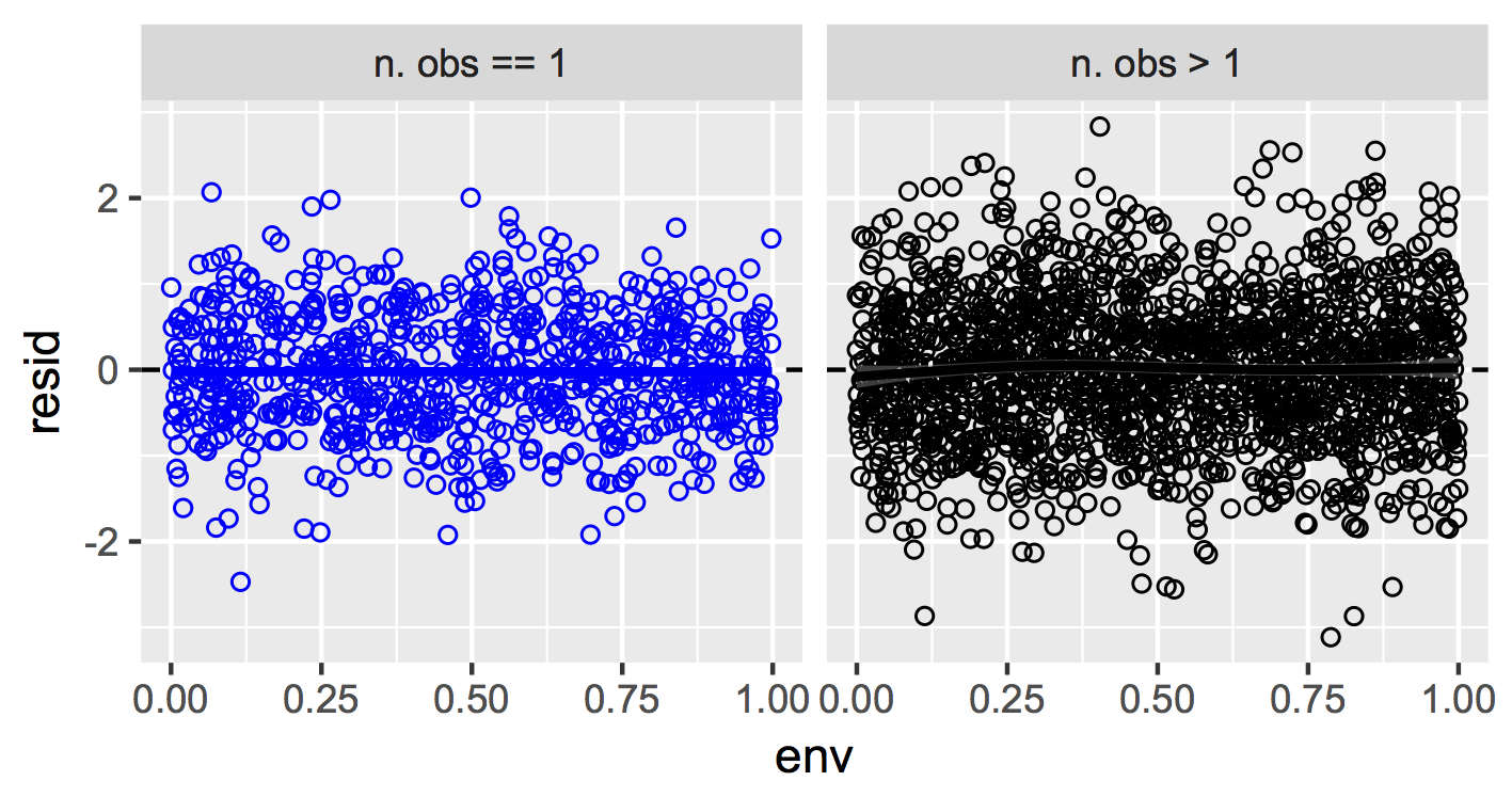
To asses the model residuals, since in this example you only have one continuous predictor, you could just plot the residuals with respect to the predictor This plot suggests that the assumptions of the linear model are respected: for example the variance of the residuals remains constant with respect to the values of the predictor, and their distribution seems symmetrical with respect to 0.