In short, your data are not normally distributed, but as long as the groups are approximately normal, you can still perform comparisons with a simple $t$-test.
Checking the normality assumption
A $t$-test requires approximate normality of the groups. You can check to see if this is reasonable to assume using a normal quantile plot, or QQ-plot. Formally testing for normality is generally not a good idea.
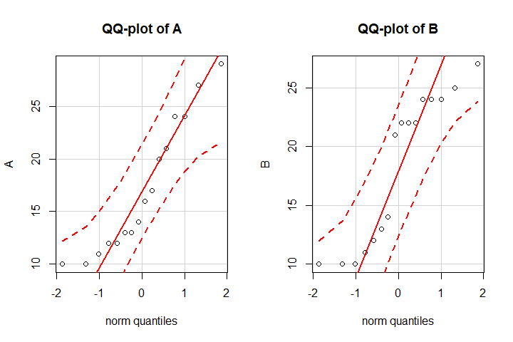
If you are using $\textsf{R}$, I recommend the qqPlot() function in car, as it includes confidence intervals by default. Using the data in your example, you can see that there is no significant deviation from normality.
A <- c(10, 12, 14, 10, 11, 12, 13, 13, 24, 24, 20, 17, 27, 16, 29, 21)
B <- c(10, 10, 21, 10, 13, 12, 22, 24, 22, 27, 24, 24, 25, 22, 11, 14)

library("car")
qqPlot(A)
qqPlot(B)

Note that this does not mean your data are normally distributed, they can't even be normally distributed, since they are integer values and the normal distribution is continuous. However, it does imply that a $t$-test is a valid way to compare these groups.
Choosing a $t$-test
An independent $t$-test requires that the observations in both groups come from distinct experimental units. This is the case when comparing A to B, but not when comparing before and after within a group. If you want to do this, you should use a paired $t$-test. For the independent $t$-test between A and B, you should also consider whether the groups' variances can be considered equal.
Lastly, if you intend to make more than one comparison, you should correct for multiple testing. A simple way to do this is by multiplying your $p$-values by the number of comparisons, known as the Bonferroni correction. Depending on what you intend to compare, this correction can easily drain power, so you could also try an FDR correction.
Alternative using regression analysis
While there are no deviations beyond the confidence intervals of the QQ-plot, notice how you can see large gap in the center of group B's QQ-plot (and more subtly in group A's), which is typical for binomial data. Since the scores are hidden ratios (number of points out of 50), a binomial regression model also makes more sense from a theoretical point of view. A more elegant way to model this would be with a binomial GLMM. In this context, you have repeated measures, which you can account for by estimating a random effect for student. In $\textsf{R}$, your model would then look something like this:
library("lme4")
GLMM <- lmer(score/50 ~ group * time + (1 | student), family = "binomial")
This does come with a slightly harder interpretation of the results if you are unfamiliar with this type of model.

