Do Likelihood Ratio Tests "respect hierarchy" in linear mixed models?

Question

The following example from the JSS paper on pkbrtest shows an LRT meant to test for the effect of the whole-plot treatment (harvest):

library("lme4")
data("beets", package = "pbkrtest")
sug <- lmer(sugpct ~ block + sow + harvest + (1 | block:harvest),
            data = beets, REML = FALSE)
sug_no.harv <- update(sug, . ~ . - harvest)
sug_no.sow <- update(sug, . ~ . - sow)

anova(sug, sug_no.harv)

At the end of Section 3.2, the authors write that, in addition to inadequacies stemming from the finite sample approximation, "the test for no effect of harvesting time is misleading because the hierarchical structure of the data has not been appropriately accounted for."

Really? But the two error terms are in there!

In this balanced data situation, a another analysis is:

beets$bh <- with(beets, interaction(block, harvest))
summary(aov(sugpct ~ block + sow + harvest + Error(bh), data = beets))

Which they claim accounts for the hierarchical structure. The p-value in the second situation is much larger, which they attribute to this.

How can the likelihood ratio test be a truly general tool if it can't test hypotheses in the presence of multiple error terms? Aside from poor finite sample size properties, is the LRT shown above logically okay?

Answer 1

The way I think about this there are several 'layers' of asymptotic adjustments going on here.

First note that the likelihood ratio test and the Wald test are asymptotically equivalent (though the LRT can be seen as a small adjustment to the Wald test to adjust for non-quadratic behavior of the log-likelihood function.) The LR and equivalent Wald tests are:

> sug <- lmer(sugpct ~ block + sow + harvest + (1 | block:harvest),
+             data = beets)
> sug_no.harv <- update(sug, . ~ . - harvest)
> anova(sug, sug_no.harv, refit=TRUE) # LR
refitting model(s) with ML (instead of REML)
Data: beets
Models:
sug_no.harv: sugpct ~ block + sow + (1 | block:harvest)
sug: sugpct ~ block + sow + harvest + (1 | block:harvest)
            Df     AIC     BIC logLik deviance  Chisq Chi Df Pr(>Chisq)    
sug_no.harv  9 -69.084 -56.473 43.542  -87.084                             
sug         10 -79.998 -65.986 49.999  -99.998 12.914      1  0.0003261 ***
---
Signif. codes:  0 ‘***’ 0.001 ‘**’ 0.01 ‘*’ 0.05 ‘.’ 0.1 ‘ ’ 1

Corresponding Wald Statistic:

> z <- coef(summary(sug))["harvestharv2", "t value"]
> z^2 # Wald chi-square statistic comparable to the LR statistic
[1] 15.21053
> pchisq(z^2, df=1, lower.tail = FALSE)
[1] 9.616582e-05
> 2 * pnorm(abs(z), lower.tail = FALSE) # equivalent
[1] 9.616582e-05

Now we can make the first finite-sample adjustment and use 20 df as we would in the corresponding fixed-effects model:

> 2 * pt(abs(z), df=20, lower.tail = FALSE)
[1] 0.0008886302

or we can take the full step and adjust for the hierarchical structure of the data and use 2 ddf:

> 2 * pt(abs(z), df=2, lower.tail = FALSE)
[1] 0.05989785

It is the latter adjustment from 20 to 2 - not the one from infinity to 20 that really matters and I think that is the one the pbkrtest authors were thinking of here. With ~200 whole plots there is no need for adjustments anymore and LR, asymptotic Wald and exact Wald (=F-test) all agree.

PS: Note that the REML LR test does not make sense because it depends on the coding of the fixed-effects in the model (and if, say, sum-to-zero contrasts are used a different test is obtained), so the LR test has to use ML -- not REML. On the other hand in the Wald test, the REML adjustment to the variance parameter estimation is important and non-ignorable given the size of this dataset: it ensures the correct variance of the harvest contrast in the example.

Answer 2

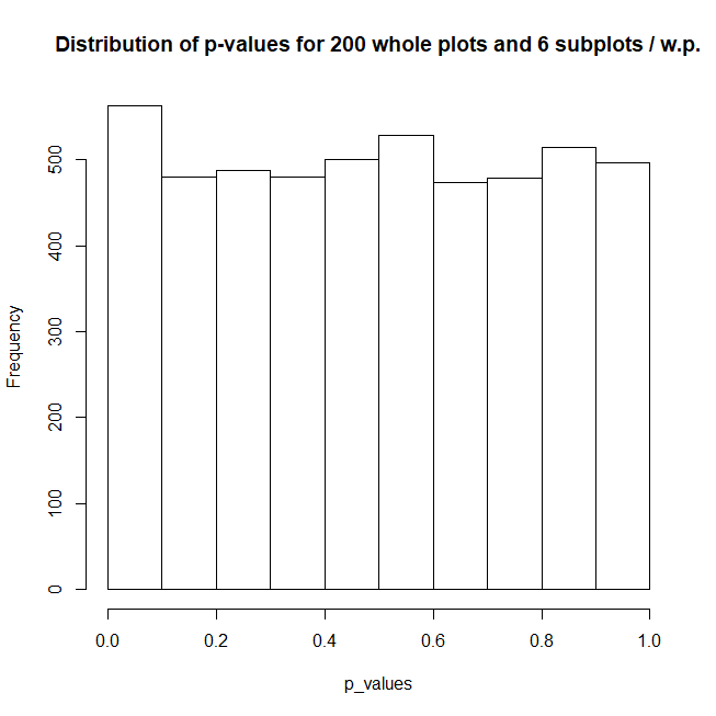
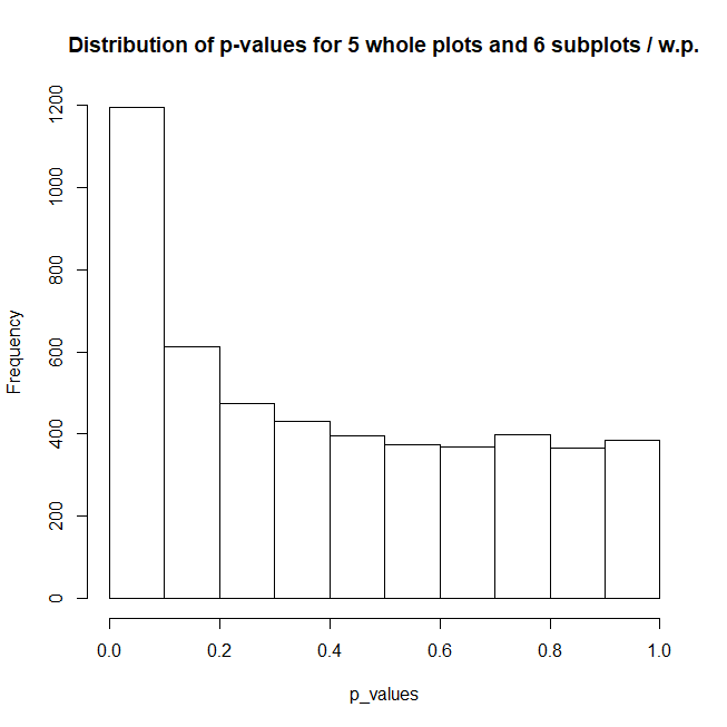
Will award best answer for theoretical justification, but a quick simulation makes me believe that the authors of pbrktest misspoke in Section 3.2. Indeed, a whole-plot treatment likelihood ratio test (LRT) is quite bad for small whole plot sample sizes, but performance improves as the number of whole plots increases. Below are whole plot p-value histograms from a Monte Carlo simulation where there is no whole plot treatment effect and we would expect a uniform distribution.

You try different whole plot and split plot sample sizes below. Of course, in an experimental design setting, the number of whole plots may indeed be small, making the methods in the pbkrtest package especially useful.

library(lme4)
set.seed(14323)

N <- 5 # whole plots. Use multiple of 2 for balanced data set
J <- 6  # subplots within w.p.s. Use multiple of 2 for balanced data set

B <- 5000 # Monte Carlo reps
p_values <- c()
for (rep in 1:B) {
  if (rep %% 100 == 0) cat("On Monte Carlo rep ", rep, "\n")
  u_i <- 5.5 * rnorm(N)
  e_i <- 2.9 * rnorm(N * J)

  sp_df <- expand.grid(subunit = 1:J, unit = 1:N)
  sp_df$wp_trt <- sp_df$unit <= N / 2
  sp_df$sp_trt <- sp_df$subunit <= J / 2

  sp_df$y <- 30 + u_i[sp_df$unit] + 1.5 * sp_df$sp_trt + e_i

  lmer_full_wp <- lmer(y ~ factor(wp_trt) + (1 | unit), data = sp_df,
                       REML = FALSE)
  lmer_red_wp <- lmer(y ~ (1 | unit), data = sp_df, REML = FALSE)

  my_anova <- anova(lmer_full_wp, lmer_red_wp)
  p_values <- c(p_values, my_anova["Pr(>Chisq)"][2, 1])
}

# With no whole plot treatment effect, the p-value distr should be uniform
hist(p_values, main = paste("Distribution of p-values for", N,
                            "whole plots", "and", J, "subplots / w.p."))