How to structure this problem in a bayesian paradigm? (Updating the posterior?)

Question

I have some code that randomly generates a number from m_min=10 to m_max=100 (apologies if this nomenclature is unconventional) for a total of (m_max - m_min) + 1 = 91 positions = n_positions each with equal probability of being picked (i.e. a uniform distribution in the form of a probability vector).

I'm running a function using each number and receiving a score, if it's better than the previous score I want to update the weights for each position. Instead of discretely updating weights, I want to also update the weights of the neighboring positions for a smooth curve.

My thoughts for implementing was to do the following:

(1) update the weights for position_k;

(2) fit curve to a beta-distribution (this part gets tricky); and then

(3) when I draw another number from m_min to m_max , call it query_num, I will divide that by n_positions (i.e. total number of positions) to get my x for the calculating the probability of drawing that value from the beta-distribution.

---

I believe this is a bayesian problem since I am using a uniform distribution as my prior and updating the posterior to get a beta-distribution (if this is incorrect, please inform me).

I am clearly missing a fundamental step in the logic.

My ultimate goal is to "update" the posterior each time the condition == True by adding mass to the regions around query_num, recompute the probabilities based on a beta distribution, and, in this case, plot the transformation.

I can't use a simple stats.beta.fit because I don't have draws from the distribution only probabilities for of the x values that I am updating.

import sys
import matplotlib.pyplot as plt
import seaborn as sns
import numpy as np
from scipy import stats
from scipy.optimize import curve_fit

# Defaults
m_min = 10
m_max = 100

# Uniform probabilities
n_positions = m_max - m_min + 1
positions = np.arange(m_min, m_max + 1)
x = np.linspace(0,1,n_positions)
# Prior probabilities
probs_num = np.ones(n_positions)/n_positions # Each value is 0.01098901

# Placeholder function
def func(x):
    # This isn't actually what I'm doing but just to get the code to work for this example
    return 15 < x < 30


# Plot updates
n_iter = 100
update_value = 1e-3
with plt.style.context("seaborn-white"):
    fig, ax = plt.subplots()
    ax.plot(x, probs_num, label="Prior", color="black")
    for i, color in enumerate(sns.color_palette(n_colors=n_iter)):
        rs = np.random.RandomState(i)
        # Get index of the position vector which is why I'm subtract `m_min`
        query_num = rs.choice(positions, size=1, replace=False, p=probs_num)[0] - m_min 
        # Again the actual conidition is more complicated
        condition = func(query_num)
        # If it meets the criteria then update the "mass" in this area of the distribution
        if condition:
            probs_num[query_num] += update_value
            # Normalize the values to probabilities again
            probs_num = probs_num/probs_num.sum()
            # Fit the curve to beta distribution (this is where it gets messed up)
            params_fitted, _ = curve_fit(lambda x,a,b:stats.beta.pdf(x, a, b), 
                                         xdata=x,
                                         ydata=probs_num,
                                        )
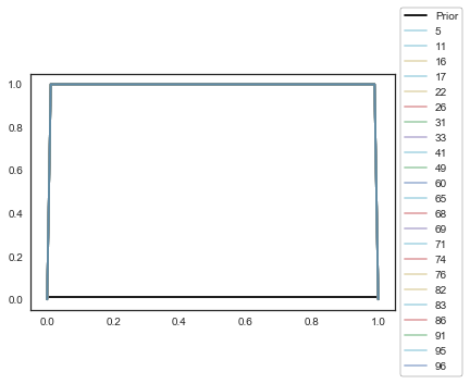
            ax.plot(x, stats.beta(*params_fitted).pdf(x), color=color, alpha=0.5, label=i)
legend_kws = {'bbox_to_anchor': (1, 0.5), 'edgecolor': 'black', 'facecolor': 'white', 'fontsize': 10, 'frameon': True, 'loc': 'center left'}          
ax.legend(**legend_kws)

Versions:

Python v3.6.4, NumPy v1.14.2, SciPy v1.0.1

Answer 1

I'm going to show you how to do this despite the fact that I'm not entirely convinced that it's the best approach. I'd like to suggest instead that you use a flexible regression model to fit the data instead. One that could be useful is Gaussian Process regression. Fitting a Gaussian Process regression model achieves your goal of "updating the weights for neighboring positions using a smooth curve". Additionally you very easily can get estimates on the uncertainty for unknown observations.

But anyway, let's proceed with what you asked. Let's set up the model you're seeking to fit. Your model is: $$x_i \sim Beta(\alpha, \beta)$$ for some $\alpha, \beta$.

Additionally, you have strong prior belief that the distribution over the data is uniform. A $Beta(1,1)$ distribution is uniform, so we need our priors on $\alpha, \beta$ to have mass near 1.

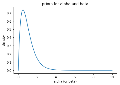
I went with $Gamma(2,2)$ priors for both $\alpha$ and $\beta$ because this distribution is defined for the positive reals (as these parameters ought to be). The choice of prior should be chosen carefully, this is just for example

import scipy.stats as ss
import bumpy as np

hyperparam_x_grid = np.linspace(0, 10, 1000)
fig, ax = plt.subplots(1,1)
rv = ss.gamma(2, scale = 1 / 2.)
density = rv.pdf(hyperparam_x_grid)
ax.plot(hyperparam_x_grid, density)
plt.title('priors for alpha and beta')
plt.xlabel('alpha (or beta)')
plt.ylabel('density')

As we can see, most of the mass of the prior is near 1 and the prior has a mean of 1.

print('prior mean for alpha and beta: {}'.format(rv.mean()))

Now we need to construct some data. Our data should be structured as a collection of points where func(x) equals 1. This is a limitation of this approach, it can't model functions where the response is not 0/1. I'm going to take every integer from the defined region (15, 35) as the sample and will illustrate how the model learns from successive points.

m_min, m_max = 10, 90
scale_func = lambda x: (x-m_min)/(m_max-m_min)
inv_scale_func = lambda x: x*(m_max-m_min)+m_min

assert all([np.isclose(inv_scale_func(scale_func(x)),x) for x in range(10, 90)])

observed_data = [scale_func(xi) for xi in range(15, 36)]

I chose PyMC3 for the probabilistic programming. We can construct our prior model (the model without observing any data) as below:

import pymc3 as pm

prior_model = pm.Model()
with prior_model:
    alpha_var = pm.Gamma('alpha', 2, 2)
    beta_var = pm.Gamma('beta', 2, 2)
    x_ = pm.Beta('x_', alpha = alpha_var, beta = beta_var)

    step = pm.NUTS() # sampler
    trace = pm.sample(15000, step)

After fitting the prior model and running the sampler, we can summarize the "posterior" for the parameters and see that we're just sampling from the priors for alpha and beta.

pm.summary(trace[-5000:])

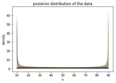
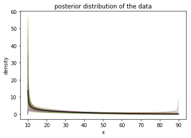
(Output not shown), but note how the mean for alpha and beta are each approximately 1. We can visualize what this looks like in terms of our data by plotting samples from the "posterior" for our data. The posterior mean is the black line, samples are transparent and colored.

def plot_posterior(trace):
    x_grid = np.linspace(0, .999, 1000)
    fig, ax = plt.subplots(1,1)
    for _ in range(100):
        i = random.randint(0, 5000)
        alpha_, beta_ = trace[-i]['alpha'], trace[-i]['beta']
        rv = ss.beta(alpha_, beta_)
        ax.plot([inv_scale_func(x) for x in x_grid],
            rv.pdf(x_grid),
        alpha  = .2)
    alpha_mean = np.mean(trace[-5000:]['alpha'])
    beta_mean = np.mean(trace[-5000:]['beta'])
    rv = ss.beta(alpha_mean, beta_mean)
    ax.plot([inv_scale_func(x) for x in x_grid], rv.pdf(x_grid), 'k')
    plt.title('posterior distribution of the data')
    plt.xlabel('x')
    plt.ylabel('density')

plot_posterior(trace)

And as desired, the prior distribution is flat without seeing any data.

Let's see what happens if we pass one data point at 15:

model_1 = pm.Model()
with model_1:
    alpha = pm.Gamma('alpha', 2, 2)
    beta = pm.Gamma('beta', 2, 2)
    x = pm.Beta('x', alpha = alpha, beta = beta, observed=observed_data[0])

    step = pm.NUTS()
    trace = pm.sample(15000, step)


pm.summary(trace[-5000:])
plot_posteriorterior(trace)

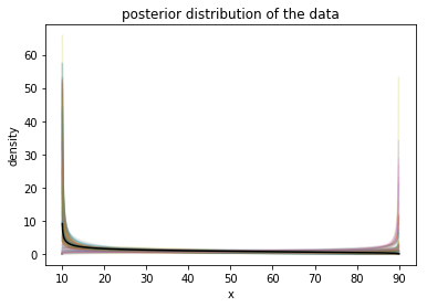
The model has updated a bit and learned that lower values are more likely. Let's see what it looks like after a few data points:

model_2 = pm.Model()
with model_2:
    alpha = pm.Gamma('alpha', 2, 2)
    beta = pm.Gamma('beta', 2, 2)
    x = pm.Beta('x', alpha = alpha, beta = beta, observed=observed_data[:5])

    step = pm.NUTS()
    trace = pm.sample(15000, step)

pm.summary(trace[-5000:])
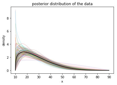
plot_posterior(trace)

Still not a great fit, possibly because of the Beta distribution or because of our strong prior. Not sure. Let's run on the full dataset:

model_full = pm.Model()
with model_full:
    alpha = pm.Gamma('alpha', 2, 2)
    beta = pm.Gamma('beta', 2, 2)
    x = pm.Beta('x', alpha = alpha, beta = beta, observed=observed_data[:5])

    step = pm.NUTS()
    trace = pm.sample(15000, step)

pm.summary(trace[-5000:])
plot_posterior(trace)

And there you have it. Your posterior distribution for the data given a Beta model. Not a great fit, to be sure, but a fit.