(Moved from comments to an answer as requested by @Greenparker)
Part 1)
The $\sqrt{\log p}$ term comes from (Gaussian) concentration of measure. In particular, if you have $p$ IID Gaussian random variables[F1], their maximum is on the order of $\sigma\sqrt{\log p}$ with high probability.
The $n^{-1}$ factor just comes fact you are looking at average prediction error - i.e., it matches the $n^{-1}$ on the other side - if you looked at total error, it wouldn't be there.
Part 2)
Essentially, you have two forces you need to control:
- i) the good properties of having more data (so we want $n$ to be big);
- ii) the difficulties have having more (irrelevant) features (so we want $p$ to be small).
In classical statistics, we typically fix $p$ and let $n$ go to infinity: this regime is not super useful for high-dimensional theory because it is (asymptotically) in the low-dimensional regime by construction.
Alternatively, we could let $p$ go to infinity and $n$ stay fixed, but then our error just blows up as the problem becomes essentially impossible. Depending on the problem, the error may go to infinity or stop at some natural upper bound (e.g., 100% misclassification error).
Since both of these cases are a bit useless, we instead consider $n, p$ both going to infinity so that our theory is both relevant (stays high-dimensional) without being apocalyptic (infinite features, finite data).
Having two "knobs" is generally harder than having a single knob, so we fix $p=f(n)$ for some fixed $f$ and let $n$ go to infinity (and hence $p$ goes to infinity indirectly).[F2] The choice of $f$ determines the behavior of the problem. For reasons in my answer to part 1, it turns out that the "badness" from the extra features only grows as $\log p$ while the "goodness" from the extra data grows as $n$.
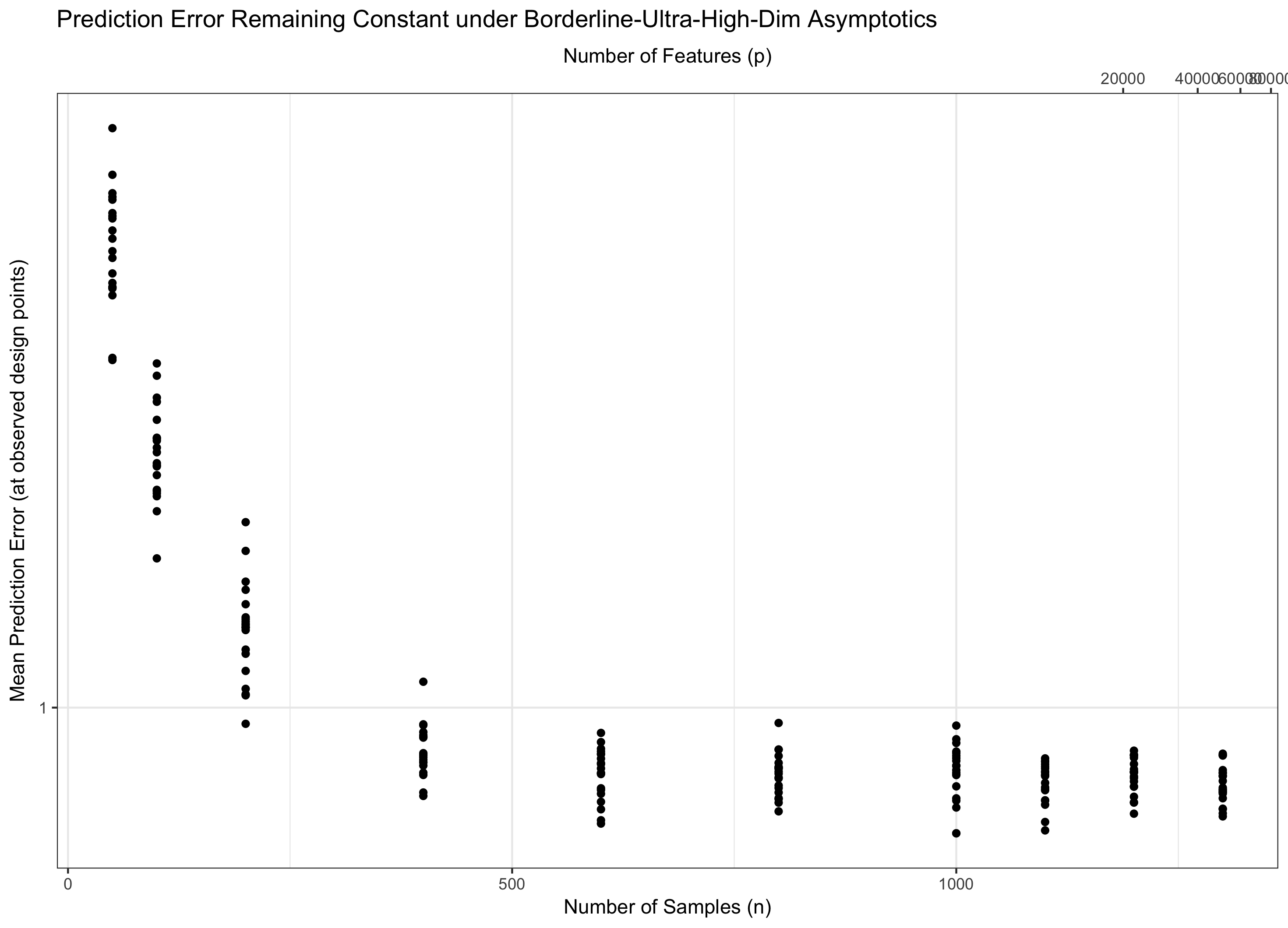
- If $\frac{\log p}{n}$ stays constant (equivalently, $p=f(n)=Θ(C^n)$ for some $C$), we tread water and the problem is a wash (error stays fixed asymptotically);
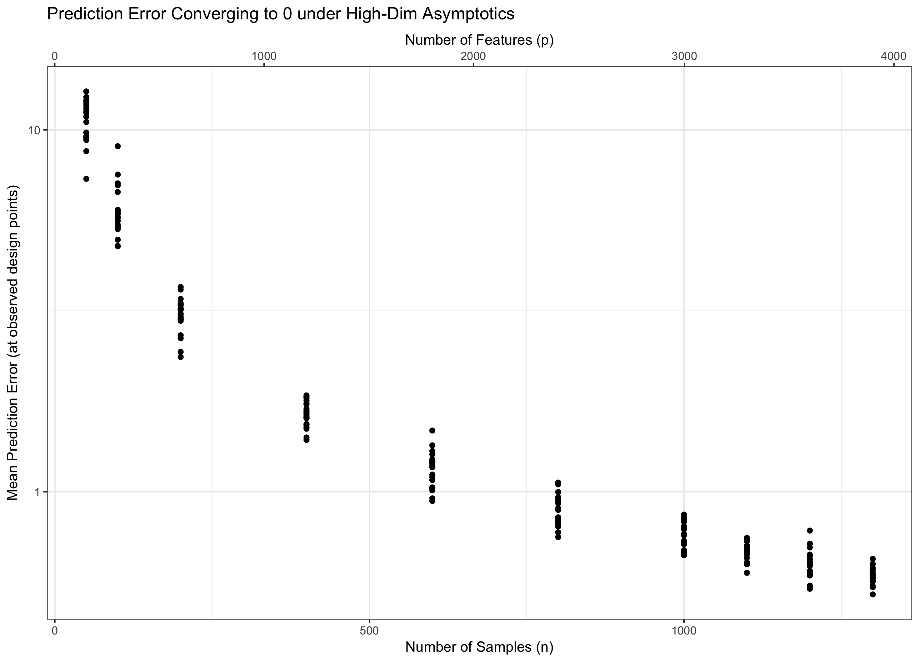
- if $\frac{\log p}{n} \to 0$ ($p=o(C^n)$) we asymptotically achieve zero error;
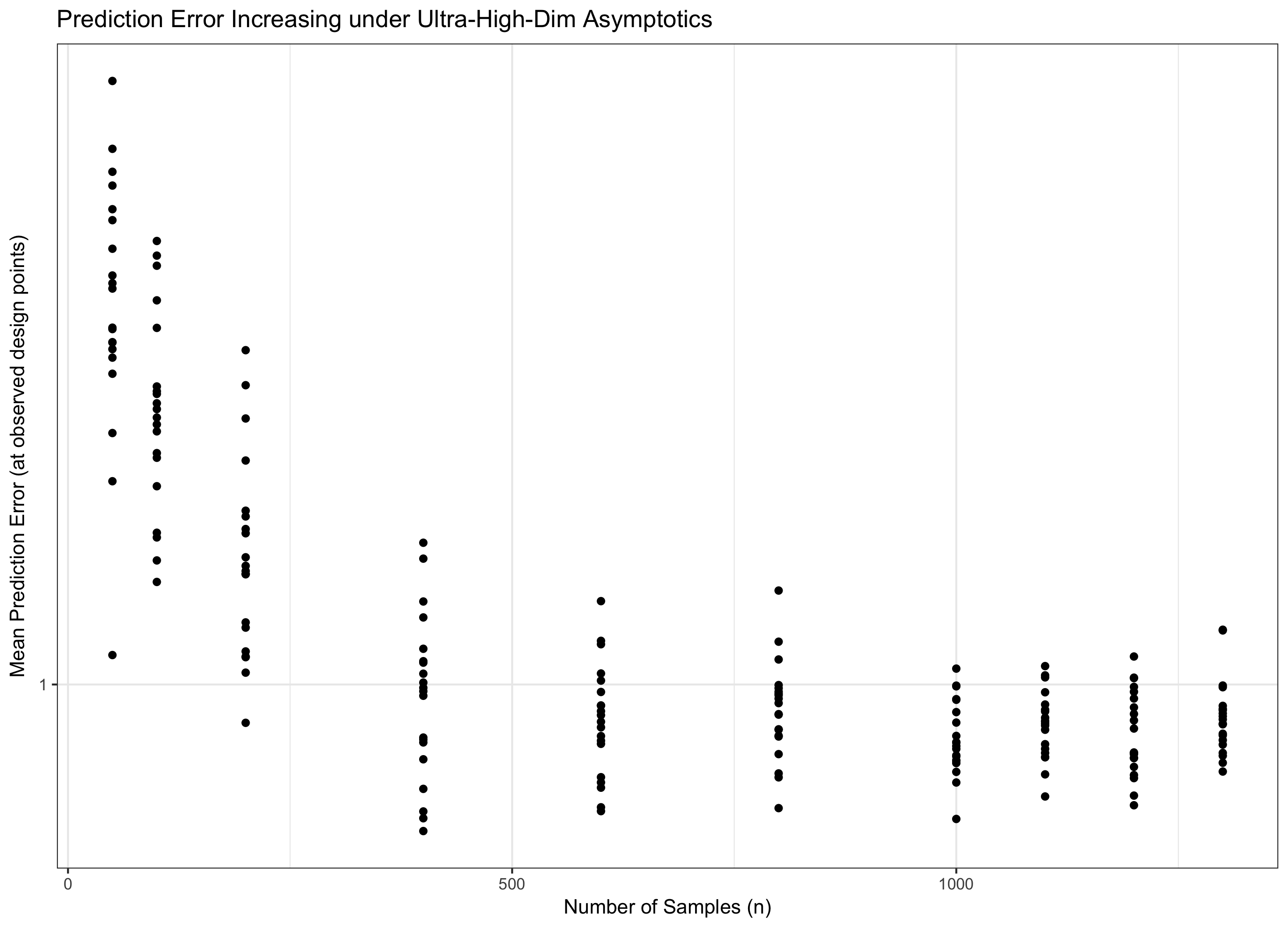
- and if $\frac{\log p}{n}→\infty$ ($p=\omega(C^n)$), the error eventually goes to infinity.
This last regime is sometimes called "ultra-high-dimensional" in the literature. The term "ultra-high-dimensional" doesn't have a rigorous definition as far as I know, but it's informally just "the regime that breaks the lasso and similar estimators."
We can demonstrate this with a small simulation study under fairly idealized conditions. Here we take theoretical guidance on the optimal choice of $\lambda$ from [BRT09] and pick $\lambda = 3 \sqrt{\log(p)/n}$.
First consider a case where $p = f(n) = 3n$. This is in the 'tractable' high-dimensional regime described above and, as theory predicts, we see the prediction error converge to zero:

Code to reproduce:
library(glmnet)
library(ggplot2)

# Standard High-Dimensional Asymptotics: log(p) / n -> 0

N <- c(50, 100, 200, 400, 600, 800, 1000, 1100, 1200, 1300)
P <- 3 * N

ERROR_HD <- data.frame()

for(ix in seq_along(N)){
  n <- N[ix]
  p <- P[ix]

  PMSE <- replicate(20, {
    X <- matrix(rnorm(n * p), ncol=p)
    beta <- rep(0, p)
    beta[1:10] <- runif(10, 2, 3)
    y <- X %*% beta + rnorm(n)

    g <- glmnet(X, y)

    ## Cf. Theorem 7.2 of Bickel et al. AOS 37(4), p.1705-1732, 2009.
    ## lambda ~ 2*\sqrt{2} * \sqrt{\log(p)/n}
    ## is good scaling for controlling prediction error of the lasso
    err <- X %*% beta - predict(g, newx=X, s=3 * sqrt(log(p)/n))
    mean(err^2)
  })

  ERROR_HD <- rbind(ERROR_HD, data.frame(PMSE=PMSE, n=n, p=p))
}

ggplot(ERROR_HD, aes(x=n, y=PMSE)) + geom_point() + theme_bw() +
xlab("Number of Samples (n)") +
ylab("Mean Prediction Error (at observed design points)") +
ggtitle("Prediction Error Converging to 0 under High-Dim Asymptotics") +
scale_x_continuous(sec.axis = sec_axis(~ 3 * ., name="Number of Features (p)")) +
scale_y_log10()
We can compare this to the case where $\frac{\log p}{n}$ stays approximately constant: I call this the "borderline" ultra-high-dimensional regime, but that's not a standard term:
P <- 10 + ceiling(exp(N/120))
Here we see that the prediction error (using the same design as above) levels off instead of continuing to zero.

If we set $P$ to grow faster than $e^n$, (e.g., $e^{n^2}$), the prediction error increases without bound. These $e^{n^2}$ is ludicrously fast and leads to enormous problems / numerical problems, so here's a slightly slower, but still UHD example:
P <- 10 + ceiling(exp(N^(1.03)/120))

(I used a sparse random $X$ for speed, so don't try to compare the numbers with the other plots directly) It's hard to see any uptick in this graph, perhaps because we kept the UHD growth from being too "ultra" in the name of computational time. Using a larger exponent (like $e^{n^1.5}$) would make the asymptotic growth a bit clearer.
Despite what I said above and how it may appear, the ultra-high-dimensional regime is not actually completely hopeless (though it's close), but it requires much more sophisticated techniques than just a simple max of Gaussian random variables to control the error. The need to use these complex techniques is the ultimate source of the complexity you note.
There's no particular reason to think that $p, n$ should grow "together" in any way (i.e., there's not an obvious "real-world" reason to fix $p = f(n)$), but math generally lacks language and tools for discussing limits with two "degrees of freedom" so it's the best we can do (for now!).
Part 3)
I'm afraid I don't know any books in the statistical literature that really focus on the growth of $\log p$ vs $n$ explicitly. (There may be something in the compressive sensing literature)
My current favorite reference for this kind of theory is Chapters 10 and 11 of Statistical Learning with Sparsity [F3] but it generally takes the approach of considering $n, p$ fixed and giving finite-sample (non-asymptotic) properties of getting a "good" result. This is actually a more powerful approach - once you have the result for any $n, p$, it's easy to consider the asymptotics - but these results are generally harder to derive, so we currently only have them for lasso-type estimators as far as I know.
If you're comfortable and willing to delve into research literature, I'd look at works by Jianqing Fan and Jinchi Lv, who have done most of the foundational work on ultra-high-dimensional problems. ("Screening" is a good term to search on)
[F1] Actually, any subgaussian random variable, but this doesn't add that much to this discussion.
[F2] We might also set the "true" sparsity $s$ to depend on $n$ ($s = g(n)$) but that doesn't change things too much.
[F3] T. Hastie, R. Tibshirani, and M. Wainwright. Statistical Learning with Sparsity. Monographs on Statistics and Applied Probability 143. CRC Press, 2015. Available at for free download at https://web.stanford.edu/~hastie/StatLearnSparsity_files/SLS.pdf
[BRT] Peter J. Bickel, Ya'acov Ritov, and Alexandre B. Tsybakov. "Simultaneous Analysis of Lasso and Dantzig Selector." Annals of Statistics 37(4), p. 1705-1732, 2009. http://dx.doi.org/10.1214/08-AOS620

