You need to fit these binned data with some distributional model, for that is the only way to extrapolate into the upper quartile.
A model
By definition, such a model is given by a cadlag function $F$ rising from $0$ to $1$. The probability it assigns to any interval $(a,b]$ is $F(b)-F(a)$. To make the fit, you need to posit a family of possible functions indexed by a (vector) parameter $\theta$, $\{F_\theta\}$. Assuming that the sample summarizes a collection of people chosen randomly and independently from a population described by some specific (but unknown) $F_\theta$, the probability of the sample (or likelihood, $L$) is the product of the individual probabilities. In the example, it would equal
$$L(\theta) = (F_\theta(8) - F_\theta(6))^{51} (F_\theta(10) - F_\theta(8))^{65} \cdots (F_\theta(\infty) - F_\theta(16))^{182}$$
because $51$ of the people have associated probabilities $F_\theta(8) - F_\theta(6)$, $65$ have probabilities $F_\theta(10) - F_\theta(8)$, and so on.
Fitting the model to the data
The Maximum Likelihood estimate of $\theta$ is a value which maximizes $L$ (or, equivalently, the logarithm of $L$).
Income distributions are often modeled by lognormal distributions (see, for example, http://gdrs.sourceforge.net/docs/PoleStar_TechNote_4.pdf). Writing $\theta = (\mu,\sigma)$, the family of lognormal distributions is
$$F_{(\mu, \sigma)}(x) = \frac{1}{\sqrt{2\pi}}\int_{-\infty}^{(\log(x)-\mu)/\sigma} \exp(-t^2/2) dt.$$
For this family (and many others) it is straightforward to optimize $L$ numerically. For instance, in R we would write a function to compute $\log(L(\theta))$ and then optimize it, because the maximum of $\log(L)$ coincides with the maximum of $L$ itself and (usually) $\log(L)$ is simpler to calculate and numerically more stable to work with:
logL <- function(thresh, pop, mu, sigma) {
  l <- function(x1, x2) ifelse(is.na(x2), 1, pnorm(log(x2), mean=mu, sd=sigma))
                        - pnorm(log(x1), mean=mu, sd=sigma)
  logl <- function(n, x1, x2)  n * log(l(x1, x2))
  sum(mapply(logl, pop, thresh, c(thresh[-1], NA)))
}

thresh <- c(6,8,10,12,14,16)
pop <- c(51,65,68,82,78,182)
fit <- optim(c(0,1), function(theta) -logL(thresh, pop, theta[1], theta[2]))
The solution in this example is $\theta = (\mu,\sigma)=(2.620945, 0.379682)$, found in the value fit$par.
Checking model assumptions
We need at least to check how well this conforms to the assumed lognormality, so we write a function to compute $F$:
predict <- function(a, b, mu, sigma, n) {
  n * ( ifelse(is.na(b), 1, pnorm(log(b), mean=mu, sd=sigma))
        - pnorm(log(a), mean=mu, sd=sigma) )
It is applied to the data to obtain the fitted or "predicted" bin populations:
pred <- mapply(function(a,b) predict(a,b,fit$par[1], fit$par[2], sum(pop)),
               thresh, c(thresh[-1], NA))
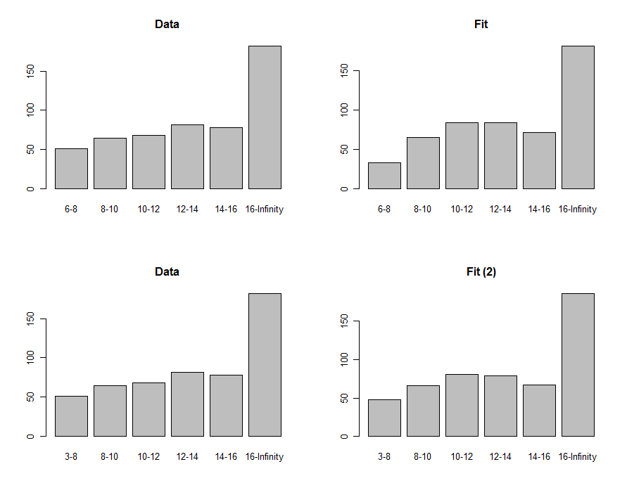
We can draw histograms of the data and the prediction to compare them visually, shown in the first row of these plots:

To compare them, we can compute a chi-squared statistic. This is usually referred to a chi-squared distribution to assess significance:
chisq <- sum((pred-pop)^2 / pred)
df <- length(pop) - 2 - 1
pchisq(chisq, df, lower.tail=FALSE)
The "p-value" of $0.0035$ is small enough to make many people feel the fit isn't good. Looking at the plots, the problem evidently focuses in the lowest $6-8$ bin. Perhaps the lower terminus should have been zero? If, in an exploratory fashion, we were to reduce the $6$ to anything less than $3$, we would obtain the fit shown in the bottom row of plots. The chi-squared p-value is now $0.26$, indicating (hypothetically, because we're purely in an exploratory mode now) that this statistic finds no significant difference between the data and the fit.
Using the fit to estimate quantiles
If we accept, then, that (1) the incomes are approximately lognormally distributed and (2) the lower limit of the incomes is less than $6$ (say $3$), then the maximum likelihood estimate is $(\mu, \sigma)$ = $(2.620334, 0.405454)$. Using these parameters we can invert $F$ to obtain the $75^{\text{th}}$ percentile:
exp(qnorm(.75, mean=fit$par[1], sd=fit$par[2]))
The value is $18.06$. (Had we not changed the lower limit of the first bin from $6$ to $3$, we would have obtained instead $17.76$.)
These procedures and this code can be applied in general. The theory of maximum likelihood can be further exploited to compute a confidence interval around the third quartile, if that is of interest.

