What explains a sudden change in the magnitude of logistic regression coefficients when increasing the sample size

Question

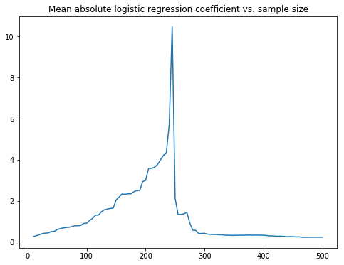
Last week my team and I discovered a strange phenomenon with the coefficients of a logistic regression (LR). As we included more samples from a static dataset, the magnitude of the coefficients of the LR kept on growing, until a certain size. After that, the magnitudes decrease rapidly.

We thought this had something to do a with a peculiarity in our dataset, with the amount of regularisation or with the visualisation itself. But after a while we replicated the phenomenon with randomly initialised data (see below).

What causes this strange behaviour of LR coefficients? Is it possible to determine the transition point (it to occur at a stable dataset size)?

Note: we use very little regularisation (C=1000).

Reproducible example

Preparation, specify number of rows N and dimension D

from sklearn.linear_model import LogisticRegression
import pandas as pd

N = 500
D = 100
sigma = 1

Generate some random data. X is an NxD array of N(0, 1) distributed data. Y is a Nx1 array of ground truth labels. model specifies the relation between X (+ noise) and Y, it has coefficients between -10 and 10.

X = pd.np.random.randn(N, D)
model = pd.np.random.randint(-10, 10, (D, 1))
noise = pd.np.random.randn(N, D) * sigma
Y = ((X + noise).dot(model) > 0).squeeze()

The next code fits a logistic regression model to subsets of the whole data. The size of the subsets increases from 10 data points to all 500 data points. For each subset the coefficients of the logistic regression are saved.

def lr_coefficients_for(sample_size):
    lr = LogisticRegression(penalty='l2', C=1000).fit(X[:sample_size,], Y[:sample_size])
    return lr.coef_

coefficients = pd.np.concatenate(list(map(lr_coefficients_for, sample_sizes)))

The mean absolute coefficient for each of the subsets is computed and plotted.

sample_sizes = range(10, N+1, 5)
pdf_coefs = pd.Series(pd.np.abs(coefficients).mean(axis=1), index=sample_sizes, name='Mean absolute coefficient')
pdf_coefs.plot(figsize=(8, 6), title='Mean absolute logistic regression coefficient vs. sample size')

The result

The image shows how the magnitude of the coefficients increase when the subset has 250 or less data points. When the number of data points gets larger than 250, suddenly the magnitude of coefficients decreases.

Answer 1

My sense is that this represents what you might expect with overfitting of a model, perhaps with some near-perfect separation added in.

A useful rule of thumb to avoid overfitting in logistic regression is to have 15 to 20 events per predictor. "Events" in this context represents the number of cases in the sample with the lower prevalence of the 2 classes. With 10 predictors in your model and as I understand it a 50/50 split of the 2 classes, then you would want 300 - 400 cases total to avoid overfitting. This is in the range where the sum of the absolute values of coefficients in your example has stabilized at a low value.

My guess is that something related to perfect separation or the Hauck-Donner phenomenon accounts for the peak at intermediate sample sizes. At very low sample sizes you do not have enough cases to find any substantial relations of classes to predictors. But at intermediate sample sizes you might pick up combinations of predictors that happen to do very well on the particular sample at hand but do not generalize well to new samples; thus the large-magnitude apparent coefficients fade away as more cases are considered.