Assuming that behavioral scores $(x)$ are numeric as well as test scores $(y)$, the short answer is that I think it would be better to do a regression of $y$ on $x.$
Regression. To illustrate, I generated fake data for 100 imaginary students. Roughly speaking, you might think of $x$'s as reported hours
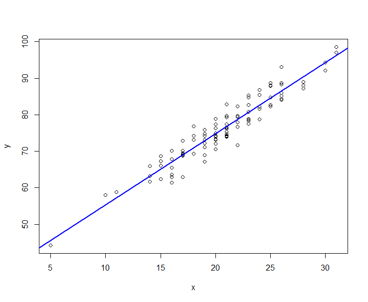
of study a week in all subjects and $y$'s as test scores. Here is a scatterplot
of the data along with the regression line.
set.seed(824)
x = round(rnorm(100, 20, 5));  e = rnorm(100, 0, 3);  y = 35 + 2*x + e
regr = lm(y ~ x)
plot(x, y);  abline(regr, lwd=2, col="blue")

Without going into all of the details about regression, I mention that one of its
advantages here is that you have an estimated regression line that fairly
accurately quantifies the relationship between $y$ and $x.$ The approximate equation is $\hat y_i = 35.87 + 1.95x,$ which might be interpreted to suggest
that each extra hour of study tends to raise an (imaginary) student's exam score by about
two points. Also the very highly significant positive slope (coefficient of $x)$
makes it clear that the two variables are significantly correlated. (Of course for real students, there are many factors in addition to
study hours that affect exam scores, and you should not expect such a clear-cut
result.)
summary(regr)

Call:
lm(formula = y ~ x)

Residuals:
   Min     1Q Median     3Q    Max
-7.053 -1.927 -0.133  2.138  6.615

Coefficients:
            Estimate Std. Error t value Pr(>|t|)
(Intercept)  35.8705     1.3209   27.16   <2e-16 ***
x             1.9478     0.0622   31.32   <2e-16 ***
---
Signif. codes:  0 ‘***’ 0.001 ‘**’ 0.01 ‘*’ 0.05 ‘.’ 0.1 ‘ ’ 1

Residual standard error: 2.785 on 98 degrees of freedom
Multiple R-squared:  0.9092,    Adjusted R-squared:  0.9082
F-statistic: 980.7 on 1 and 98 DF,  p-value: < 2.2e-16
Two-sample tests on 'tails'. Towards an answer of the specific question you asked, you could easily find
the study hours x.LO of the 25 students with the lowest exam scores and the
the study hours x.HI if the 25 students with the highest exam scores,
and compare them using a two-sample test.
quantile(y)
      0%      25%      50%      75%     100%
44.25723 70.14542 76.21789 82.66887 98.51916
x.LO = x[y<70.15]; x.HI = x[y > 82.67]
length(x.HI)
[1] 25
length(x.LO)
[1] 25

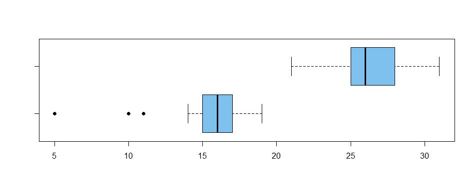
boxplot(x.LO, x.HI, col="skyblue2", pch=19, horizontal=T)

These two groups clearly have different numbers of study hours per week.
For real students, the separation would likely not be as complete as here,
but possibly strong enough to find a significant difference in study hours
using a two-sample test. The question is, which two-sample test.
Welch t test: Because we are looking at the two tails of a distribution, the data are not
likely to be normal. (For example, the observations in x.LO fail a Shapiro-Wilk normality
test shapiro.test(x.LO) with P-value 0.0003.) Nevertheless, a Welch separate-variances t test t.test(x.LO), x.HI) found a significant difference
with P-value very near $0.$
Wilcoxon rank sum test: I cannot think of any argument whereby the x.HI population could be considered
'shifted' from the x.HI population because they clearly have different shapes.
Nevertheless, a Wilcoxon rank sum test wilcox.test(x.L0, x.HI) found a
significant difference between the samples with a P-value very near $0,$
along with a warning about tied observations that one can ignore here.
Permutation test: If there were strong indications against doing either a t test or a Wilcoxon rank sum test, then you could do a permutation test.
(Omitted here, but you can search for 'permutation test' online or look at this Q&A and its references.)
Finally, before selecting any two-sample test you should consider why you would
want to discard particular information on half of your subjects when your goal is to explore the connection between $x$'s and $y$'s. Is there some reason you are interested only in the students who are extreme in some sense? (I think this was
the main point of @Glen_b's Comment.) If I do a regression only on the half of
the data you would discard, I still get a highly significant and useful linear relationship between the two variables.
Caution about fake data. With real data on real students, it would be entirely possible to get useful
results from a simple linear regression, and yet find no difference in
behavior scores with any of the two-sample tests mentioned above. All it would take for that to happen would be a somewhat lower correlation between $x$'s and $y$'s. (There were
particular points I wanted to make along the way, so I chose fake data
that would give strong effects. The point is to think about the methods;
don't expect results from actual data to be the same.)


