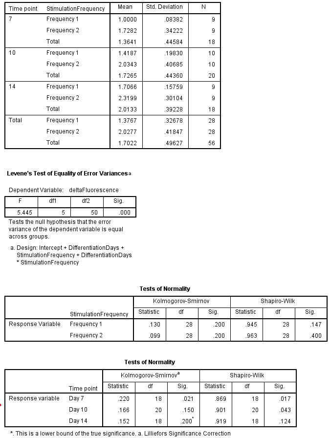
Thanks for showing key output. For several reasons, I think the
conclusions from your ANOVA are valid, even though some assumptions
are not met.
Frequency effect: First, just from the information you gave, I can see that at Time 7
Frequencies 1 & 2 differ. Because this is just a two-sample t test,
I can choose the Welch version which does not assume equal variances.
This can be done by hand from formulas, but I did it in Minitab.
You can see that this is the Welch (separate-variances) test because
DF = 8 (instead of 16). [Welch has DF between 8 and 16, lower to the extent that sample SDs differ.] Even with this "loss" of DF, the P-value is very small.
Two-Sample T-Test and CI

Sample  N    Mean   StDev  SE Mean
1       9  1.0000  0.0840    0.028
2       9   1.730   0.342     0.11


Difference = μ (1) - μ (2)
Estimate for difference:  -0.730
95% CI for difference:  (-1.001, -0.459)
T-Test of difference = 0 (vs ≠):
    T-Value = -6.22  P-Value = 0.000  DF = 8
Similarly frequencies differ very significantly at Time 10:
Two-Sample T-Test and CI

Sample  N   Mean  StDev  SE Mean
1       9  1.420  0.198    0.066
2       9  2.030  0.407     0.14


Difference = μ (1) - μ (2)
Estimate for difference:  -0.610
95% CI for difference:  (-0.942, -0.278)
T-Test of difference = 0 (vs ≠):
    T-Value = -4.04  P-Value = 0.002  DF = 11
Again at Time 14, frequencies differ very significantly. P-value < 0.0005.
Summarizing the Frequency-effect, there is no problem declaring results for Frequencies 1 and 2
to differ across time points (consistently smaller for Frequency 1) because all three P-values are so small.
If you want to compare results for several different treatment combinations,
you could look at 99% confidence intervals for pairs of the six cell means. They would
be of the form $\bar X_{ij} \pm 2.306 S_{ij}/\sqrt{9}$ or $\bar X \pm 0.77\,S_{ij}.$
For example the 99% CI for the population mean in the cell for Frequency 1 at Time 7
is $1.0 \pm 0.06.$
You could make several Bonferroni comparisons at levels around 95%.
qt(.975, 8)
[1] 2.306004
2.3/3
[1] 0.7666667
Time effect: Now for the time effect, you can do a two one-way ANOVAs with all of your data: first 27 observations for Frequency 1, then second 27 for Frequency 2. Preferably, you would use the version
that allows for unequal variances. I hope that version is available in SPSS.
However, because this is an balanced design, the standard ANOVA is easy to do based on information you provide.
For Frequency 1: MS(Factor) is the variance of the three sample means multiplied by 9. Also, MS(Error) is the mean of the three sample variances. Using R mainly as
a calculator, I got the following results. MS(Factor) = 0.6517 with DF = 2
and MS(Error) = 0.0231 with DF = 24, and F = 36.29, which greatly exceeds
the critical value 5.61 for a test at the 1% level; the P-value is less
than 0.0005.
msf = 9*var(c(1.1, 1.42, 1.71)); msf
[1] 0.8379
mse = mean(c(.084, .193, .158)^2); mse
[1] 0.02308967
f = msf/mse;
[1] 36.28896
1 - pf(f, 2, 24)
[1] 5.546266e-08
qf(.99, 2, 24)
[1] 5.613591
You can do the same for Frequency 2.
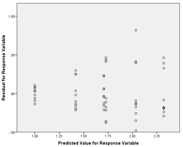
Comments on assumptions: Heteroscasticity. From your residual plot we can see that variance
differ considerably for among the $2 \times 3 = 6$ treatment combinations.
Thus it is a good idea to look at procedures that do not assume equal variances.
However, because this is a balanced design (9 replications in each cell)
and effects seem convincingly large, it seems reasonable to assume significance, if not to rely on specific difference in post-hoc tests.
As you say, you might seek a transformation to make cell variances more nearly equal, but that can make post hoc comparisons awkward.
Normality. I am not sure how SPSS does the Shapiro-Wilk test for ANOVA
designs. It would be incorrect to expect the 45 original data values to be collectively normally
distributed because, even if individually normal, they would have a mixture distribution
of normals with six potentially vary different means. (A mixture distribution of normals with different means is need not be even nearly normal.)
The correct way to
assess normality is by looking at residuals. Looking at your residual plot
I don't see departures from normality serious enough to ruin your ANOVA. You might want to test the residuals formally,
but with nine observations per cell and differences in cell mean as large
as yours I don't think the significant results of your ANOVA are in question.
Addendum: Curious to see what results for a Welch-type one-way ANOVA of various Times for Frequency 1 would give, I did a nonparametric bootstrap with data for the
three times modeled after sample means and SDs in your printout. (In R,
the procedure for a one-way ANOVA that does not assume equal variances is
oneway.test.) Sampling 100,000 datasets roughly like yours for Frequency 1,
I got an average P-value of $4.1 \times 10^{-7}$ and all P-values < 0.0005.
m = 10^5;  pv = numeric(m);  gp = as.factor(rep(c(7,10,14), each=9))
for(i in 1:m) {
  t.7 = rnorm(9, 1, .014); t.10 = rnorm(9, 1.4, .198);  t.14 = rnorm(9, 1.7, .158)
  all = c(t.7,t.10,t.14); pv[i] = oneway.test(all~gp)$p.val }
mean(pv);  mean(pv < .0005)
[1] 4.122535e-07
[1] 1
Note: I know you asked for no recommendations to use R, but this gives a
promising indication that an ANOVA you do in SPSS will give a significant result.
I would just point out that R is very good software, available without cost
at r-project.org. Some people hesitate to use R because they see so many
complicated things done with it. But there is no obligation to learn more
about R than you need for the task at hand (probably much like you're doing with SPSS), and there are numerous help sessions on line.


