2
$\begingroup$

I try to fit a random effects model for my thesis, a meta analysis of studies about team planning and team performance.

I'm using R and the package metafor to create z correlations and variance (yi, vi) and fit the model:

meta <- escalc(measure = "ZCOR",
               ri = effect,
               ni = n.teams,
               data = meta,
               slab = uid)
rma(yi, vi, data = meta)

I'm puzzled by the result:

Random-Effects Model (k = 23; tau^2 estimator: REML)

tau^2 (estimated amount of total heterogeneity): 0.0000 (SE = 0.0081)
tau (square root of estimated tau^2 value):      0.0011
I^2 (total heterogeneity / total variability):   0.00%
H^2 (total variability / sampling variability):  1.00

Test for Heterogeneity: 
Q(df = 22) = 28.0557, p-val = 0.1738

Model Results:

estimate      se    zval    pval   ci.lb   ci.ub     
  0.2542  0.0361  7.0363  <.0001  0.1834  0.3251  ***

---
Signif. codes:  0 ‘***’ 0.001 ‘**’ 0.01 ‘*’ 0.05 ‘.’ 0.1 ‘ ’ 1

Does this mean there is no heterogeneity between my studies at all? And all variability originates from sampling variability? That doesn't seem probable. Could there be a problem with my data, that causes such a result?

I tried to fit a multilevel model:

tmp <- rma.mv(yi, vi,
              random = list(~ 1 | study.id/uid),
              data = meta)
summary(tmp)

Result:

Multivariate Meta-Analysis Model (k = 23; method: REML)

  logLik  Deviance       AIC       BIC      AICc  
  2.4194   -4.8389    1.1611    4.4342    2.4945      

Variance Components: 

            estim    sqrt  nlvls  fixed        factor
sigma^2.1  0.0000  0.0000     13     no      study.id
sigma^2.2  0.0000  0.0000     23     no  study.id/uid

Test for Heterogeneity: 
Q(df = 22) = 28.0557, p-val = 0.1738

Model Results:

estimate      se    tval    pval   ci.lb   ci.ub     
  0.2542  0.0361  7.0366  <.0001  0.1793  0.3292  ***

There seems to be no variance in and between the studies.

My data:

                 uid        study.id n.teams      yi     vi
1          Lei2016.1         Lei2016      11 -0.6625 0.1250
2          Lei2016.2         Lei2016      11 -0.2661 0.1250
3          Lei2016.3         Lei2016      11 -0.6475 0.1250
4         Tasa2005.1        Tasa2005      54  0.2769 0.0196
5      Mathieu2006.1     Mathieu2006      29  0.3095 0.0385
6      Mathieu2006.2     Mathieu2006      29  0.2554 0.0385
7      Mathieu2006.3     Mathieu2006      29  0.1820 0.0385
8      Mathieu2006.4     Mathieu2006      29  0.2132 0.0385
9       Müller2009.1      Müller2009      20  0.0200 0.0588
10    Earley2000_1.1    Earley2000_1      23  0.4001 0.0500
11    Earley2000_2.1    Earley2000_2      24  0.7414 0.0476
12    DeChurch2008.1    DeChurch2008      38  0.1511 0.0286
13    DeChurch2008.2    DeChurch2008      38  0.2554 0.0286
14    DeChurch2008.3    DeChurch2008      38  0.2027 0.0286
15    DeChurch2008.4    DeChurch2008      38  0.4722 0.0286
16      Simons1999.1      Simons1999      57  0.2237 0.0185
17      Simons1999.2      Simons1999      57  0.3205 0.0185
18     Janicik2003.1     Janicik2003      48  0.4001 0.0222
19     Maynard2012.1     Maynard2012      60  0.2661 0.0175
20      Fisher2014.1      Fisher2014      32  0.2554 0.0345
21      Fisher2014.2      Fisher2014      32  0.0601 0.0345
22 vanderkleij2009.1 vanderkleij2009      36  0.1104 0.0303
23       mehta2009.1       mehta2009      91  0.3541 0.0114

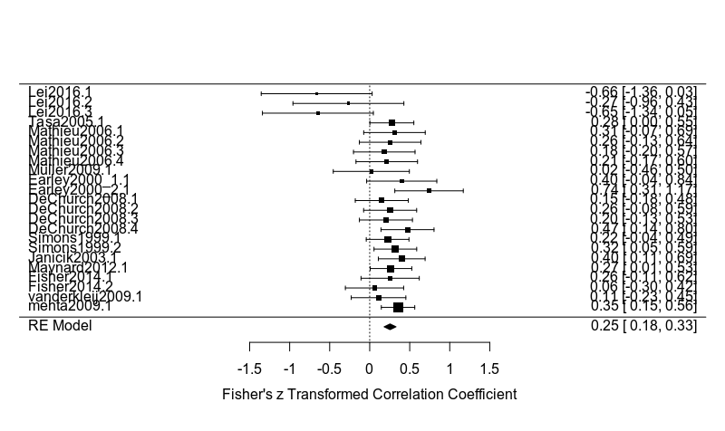
enter image description here

$\endgroup$

2 Answers 2

2
$\begingroup$

This result means that there is no more variance than you would expect by chance between the studies, and you do not have evidence for heterogeneity. This does not mean that there is no heterogeneity, just that you have failed to detect the heterogeneity.

Why does this seem unlikely to you?

How large are the samples in the studies from which you got your effect sizes?

Edit: Looking at the forest plot, there's a lot of overlap, so I'm not surprised at the lack of heterogeneity.

$\endgroup$
5
  • $\begingroup$ Thank you very much for the clarification. I added my data to the question. We investigate teams and not individuals, the sample size is the number of teams in a study. So the samples may be to small? $\endgroup$
    – Jes
    Commented Sep 13, 2018 at 15:36
  • $\begingroup$ Can you post the forest plot? $\endgroup$ Commented Sep 13, 2018 at 16:01
  • $\begingroup$ The samples may be too small to detect heterogeneity. But I don't think that's an issue or that you care very much. $\endgroup$ Commented Sep 13, 2018 at 16:06
  • $\begingroup$ I added the forest plot to the question and accepted your answer. Thank you for your time. If you think there is anything conspicuous about the forest plot, please tell me so. $\endgroup$
    – Jes
    Commented Sep 13, 2018 at 21:31
  • $\begingroup$ I was looking for a small number of studies that stood out as being clearly different. Look at the forest plot on this page: erim.eur.nl/research-facilities/meta-essentials/user-manual/… for an example of heterogeneity. $\endgroup$ Commented Sep 13, 2018 at 22:39
0
$\begingroup$

Rather than only focusing on statistical heterogeneity and inconsistency, consider checking for small study effects (e.g. publication bias). For a detailed introduction, you may read for instance Thornton and Lee.

Inspecting your forest plot, there might be indeed some publication bias.

I recommend you to provide a funnel plot and then apply a regression test (e.g. Egger's), which is easily performed in R with the funnel command and with the regtest command.

$\endgroup$

Your Answer

By clicking “Post Your Answer”, you agree to our terms of service and acknowledge you have read our privacy policy.

Not the answer you're looking for? Browse other questions tagged or ask your own question.