Random walk with "negative coefficient"

Question

I was playing around in R with simulating random walks. At some point I tried this model:

x = NULL
x[1] = 0

for (i in 2:2000) {
  x[i] = -x[i-1] + rnorm(1) 
}

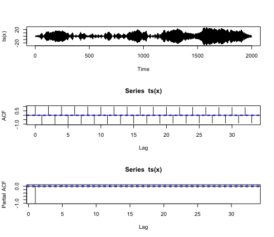
Below are a time series plot, the acf and pacf.

Now, what exactly is this? Is it also called random walk? The time series plot doesn't look like one (seems to be stable around the mean). It's not, to me, clear if the variance is increasing over time. The ACF and PACF, however, is what one might expect except for the oscillating pattern.

Is there anything concrete that can be modelled with this model?

Answer 1

To answer the variance issue, we consider

$$x_t = -x_{t-1}+u_t,\;\;\; x_1=0,\;\; u_t \sim WN(\sigma^2_u)$$

Writing recursively backwards we have

$$x_t = -x_{t-1}+u_t = -(-x_{t-2}+u_{t-1})+u_t = x_{t-2} -u_{t-1}+u_t$$

$$=-x_{t-3}+u_{t-2} -u_{t-1}+u_t = -(-x_{t-4}+u_{t-3})+u_{t-2} -u_{t-1}+u_t$$

$$= x_{t-4} - u_{t-3}+u_{t-2} -u_{t-1}+u_t$$

or

$$x_t = u_t-u_{t-1}+u_{t-2}...(-1)^{p_{t}}u_1$$

where $p_t$ here is the parity of $t$, taking the value $1$ if $t$ is an even number. regardless, the variance of the process is

$$\text{Var}(x_t) = t\cdot \sigma^2_u$$

So it has the same mean (zero), and variance as

$$x_t = \sum_{s=1}^tu_s$$

but indeed different typical evolution over time, as should be expected.

Don't expect to straightforwardly verify the "equal variances" result through sample moments, since these are not ergodic processes.