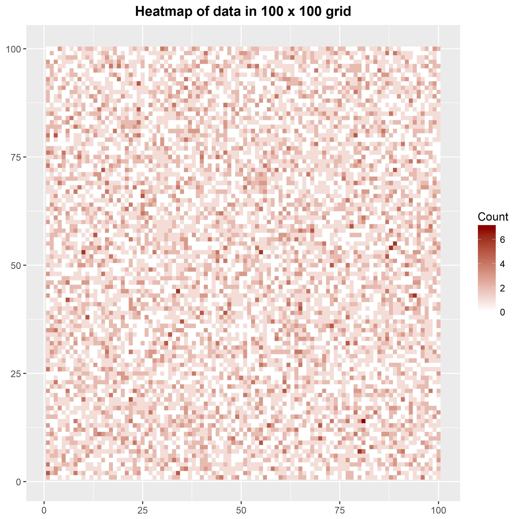
There are many kinds of tests that could potentially be done for this type of data. One possibility is to use a uniformity test based on counting the outcomes of values in a discrete grid in the space of interest. For example, if we form a square-grid over the space, we can create a $100 \times 100$ matrix counting the number of points that fall in each region.
#Count values in regions of a 100x100 grid
COUNTS <- matrix(0, nrow = 100, ncol = 100);
for (i in 1:n) { A <- ceiling(100*data$x[i]);
                 B <- ceiling(100*data$y[i]);
                 COUNTS[A,B] <- COUNTS[A,B] + 1; }

#Convert counts to data frame
CC <- data.frame(x     = rep(1:100, each = 100),
                 y     = rep(1:100, times = 100),
                 Count = rep(0, 10000));
for (i in 1:n) { CC$Count[i] <- COUNTS[CC$x[i], CC$y[i]]; }

#Plot heatmap of data
library(ggplot2);
ggplot(data = CC, aes(x = x, y = y)) +
    geom_tile(aes(fill = Count)) +
    scale_fill_gradient2(low = 'white', high = 'darkred') +
    theme(plot.title = element_text(hjust = 0.5, face = 'bold')) +
    ggtitle('Heatmap of data in 100 x 100 grid') +
    xlab(NULL) + ylab(NULL);

Occupancy test: A simple test that can be applied to count data of this kind is an occupancy test, where we count the number of grid cells that are empty and compare this to its null distribution under the hypothesis of a uniform distribution. (I make no claim to power here; the occupancy test loses quite a bit of power due to discarding information on cell count. It is presented just to give an example of a simple test.) This is done by noting that the number of empty cells follows a classical occupancy distribution. Under the alternative hypothesis of non-uniformity the number of empty cells is likely to be less than under the null hypothesis of uniformity. Hence, the p-value of the test is calculated as the probability of observing no more empty cells than was actually observed, under the null distribution.
Let $n$ be the number of data points, let $m$ be the number of cells, and let $K$ be the number of empty cells. When the number of data points and cells are both large we have the distributional approximation $n-K \sim \text{Pois}(m \cdot \exp(-n/m))$ under the null hypothesis of uniformity. Hence, we can implement the classical occupancy test as follows:
#Count cells and empty cells
m <- 10000;
K <- sum(COUNTS == 0);

#Calculate p-value of test
L <- m*exp(-n/m);
p <- ppois(K, L);

p
[1] 0.5710965
From this p-value we see that there is no evidence to reject the null hypothesis of uniformity. (Note that this is not the same as accepting uniformity - it simply means that this distributional assumption is not falsified by the occupancy test.)
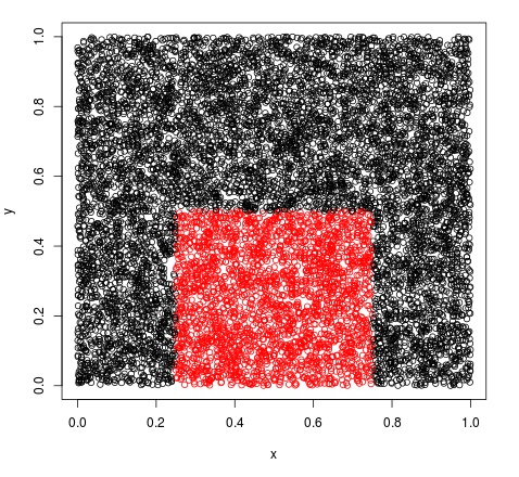
Splitting the test over two regions: If you want to separately test each of the two coloured regions in your question, this is simply a matter of performing two tests over those two regions. (Since you are now performing two tests you should be mindful of the issue of multiple comparisons.) To do this we can proceed as follows:
#Create matrix identifying the groups
GROUPS <- matrix('Black', nrow = 100, ncol = 100);
for (x in 26:75) { for (y in 1:50) { GROUPS[x,y] <- 'Red' } }

#OCCUPANCY TEST FOR BLACK GROUP
#Count data points, cells and empty cells
n <- sum(COUNTS*(GROUPS == 'Black'));
m <- sum(GROUPS == 'Black');
K <- sum((COUNTS == 0) & (GROUPS == 'Black'));

#Calculate p-value of test
L <- m*exp(-n/m);
p <- ppois(K, L);

p
[1] 0.5062172

#OCCUPANCY TEST FOR RED GROUP
#Count data points, cells and empty cells
n <- sum(COUNTS*(GROUPS == 'Red'));
m <- sum(GROUPS == 'Red');
K <- sum((COUNTS == 0) & (GROUPS == 'Red'));

#Calculate p-value of test
L <- m*exp(-n/m);
p <- ppois(K, L);

p
[1] 0.6371047
From these p-values we see that there is no evidence to reject the null hypothesis of uniformity in either group. (Again, note that this is not the same as accepting uniformity - it simply means that this distributional assumption is not falsified by the occupancy test.)


