3
$\begingroup$

I'm trying to assess the effectiveness of a program by comparing employee performance before the program vs. after the program. I have 4 years (2 years before vs. 2 years after) of individual-level employee performance data, aggregated at the monthly level. Employees could leave the company or transfer to another position, so most individuals do not have the full 48 (4*12) months of data, which leaves lots of missing values in the data set.

I looked at lots of posts and decided to use mixed model with repeated measures for this comparison.

According to answers to this post: Using lmer for repeated-measures linear mixed-effect model, I decided to configure my model as:

m1 <- lmer(Performance ~ Program + Month + Program:Month + (1+Month|Employee_Name), mydata)

Performance is a continuous variable, Program is binary (0/1) and Month is a date variable, e.g. 1/1/2016, 2/1/2016. My understanding of the equation is that: "Program : Month" allows the program has different performance across months; "1+Month/Employee_Name" allows every employee's performance to have a different intercept and coefficients.

One of my confusion is that Program and Month is correlated, with 2015-2016 months have the program (program = 1) while 2017-2018 months don't have the program (program = 0).

Regardless, I ran the model and got this warning:

singular fit Warning message: Some predictor variables are on very different scales: consider rescaling

I'm not sure how to scale the Date variable and I also researched the reason for singular fit on this post: Dealing with singular fit in mixed models

It explains "the random effects structure is too complex to be supported by the data, which naturally leads to the advice to remove the most complex part of the random effects structure (usually random slopes)."

I don't know how to address this singular issue and how to reconstruct my model to have a reasonable result.


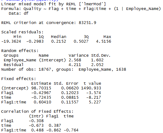
UPDATES: I changed Month to a numeric variable, starting from 0, then divided it by 12 to transform it to a year variable. I then ran the mixed model with this formula: lmer_perf <- lmer (Quality ~ Flag + time + Flag:time + (1 | Employee_Name), data = df). It does not have singular fit error!!! The formula only randoms the intercept, but I wanted to randomize the slop as well. So I constructed the below formula:

lmer_quality <- lmer (Quality ~ Flag + time + Flag:time + (1 + time | Employee_Name), data = df)

but then got this warning message: Warning message: In checkConv(attr(opt, "derivs"), opt$par, ctrl = control$checkConv, : Model failed to converge with max|grad| = 0.00722004 (tol = 0.002, component 1)

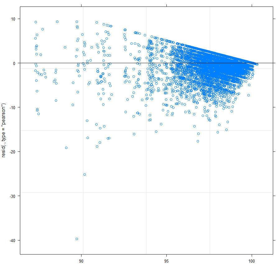
Here are the results and the residual plot from the first formula. The plot is still not good and I don't know how to interpret the results from the output.

enter image description here

enter image description here

$\endgroup$

1 Answer 1

3
$\begingroup$

A couple of points:

  • This sounds like a cross-over design in which employees are for a period on the program and then off the program. On the one hand, having each employee being its own control can increase the power. However, there are also a number of issues that you may have with such designs, such that the ordering you do things may matter (e.g., first program and the off or first off and the program). I would suggest that you search about the intricacies and analysis with such designs.
  • Your model does not sound overly complex, but you mentioned that you have the Month variable as a date variable? You should better transform it to follow-up time (by substracting the first date from all the other dates; then 0 will correspond to the first measurement).
  • Mixed models work with unbalanced data, and they provide valid inferences under the missing at random assumption if correctly specified. Hence, having less measurements for some employees may not be an issue (unless it is for missing not at random reasons).
$\endgroup$
7
  • $\begingroup$ Hi Dimitris, thank you so much for the response. While I'm researching more cross-over designs, I continued to modify the mixed model. I changed the Month variables to numeric ones starting from 0, and magically it does not give me the warning of singular fit! However I got another warning message: Some predictor variables are on very different scales: consider rescaling, and the residual plot looks very bad - small residuals at larger numbers and large residuals at smaller numbers. Do you have any advice for rescaling and improve the residual plot? $\endgroup$
    – LY1
    Commented Feb 11, 2019 at 16:32
  • $\begingroup$ It would help if you could show us the output and the residuals plot. Perhaps it has to do with the scale of your time variable, e.g, trying changing from months to years or vice versa. $\endgroup$ Commented Feb 11, 2019 at 18:15
  • $\begingroup$ I just edited the answer to include the output and the residual plot. I don't really understand why this mixed model could not handle the time variable at the monthly level.. I already converted it to numeric values starting from 0. $\endgroup$
    – LY1
    Commented Feb 12, 2019 at 4:39
  • $\begingroup$ Try working in years instead of months. Moreover, is there an upper bound in your outcome variable ‘Quality’? $\endgroup$ Commented Feb 12, 2019 at 5:38
  • $\begingroup$ Quality ranges from 0 to 100, so the upper bound is 100. To convert time to years, I need to aggregate monthly employee performance into years too. What way would you suggest aggregating monthly employee performance to years, e.g. take the mean? $\endgroup$
    – LY1
    Commented Feb 12, 2019 at 16:05

Your Answer

By clicking “Post Your Answer”, you agree to our terms of service and acknowledge you have read our privacy policy.

Not the answer you're looking for? Browse other questions tagged or ask your own question.