Studentised mean-difference: I'll start off by noting that the studentised mean-difference (SMD) for a T-test with independent samples is not what you have written. The moments of the sample mean-difference are:
$$\mathbb{E}(\bar{X}_1-\bar{X}_2) = \mu_1 - \mu_2 \quad \quad \quad
\mathbb{V}(\bar{X}_1-\bar{X}_2) = \frac{\sigma_1^2}{n_1} + \frac{\sigma_2^2}{n_2},$$
so the SMD should be:
$$T = \frac{\bar{X}_1-\bar{X}_2}{\sqrt{S_1^2/n_1 + S_2^2/n_2}}.$$
Distribution of the SMD: Unfortunately the SMD in this kind of test is not a pivotal quantity. Its distribution and its variance depend on the true distribution of the groups. You have not specified the true distribution, but I'm going to assume that you're willing to use in the special case of data from a normal distribution. In this case, we know from Cochran's theorem that the sample mean and sample variance of each group are independent, so all elements of the SMD are independent, and the distributional form is:
$$\begin{equation} \begin{aligned}
T
&= \frac{\bar{X}_1-\bar{X}_2}{\sqrt{\sigma_1^2/n_1 + \sigma_2^2/n_2}} \ \Bigg/ \ \sqrt{\frac{S_1^2/n_1 + S_2^2/n_2}{\sigma_1^2/n_1 + \sigma_2^2/n_2}} \\[12pt]
&= \frac{\bar{X}_1-\bar{X}_2}{\sqrt{\sigma_1^2/n_1 + \sigma_2^2/n_2}} \ \Bigg/ \ \sqrt{\frac{\sigma_1^2/n_1}{\sigma_1^2/n_1 + \sigma_2^2/n_2} \cdot \frac{S_1^2}{\sigma_1^2} + \frac{\sigma_2^2/n_2}{\sigma_1^2/n_1 + \sigma_2^2/n_2} \cdot \frac{S_2^2}{\sigma_2^2}} \\[12pt]
&\sim \text{N}(0,1) \ \Bigg/ \ \sqrt{\frac{\sigma_1^2/n_1}{\sigma_1^2/n_1 + \sigma_2^2/n_2} \cdot \frac{\text{Chi-Sq}(n_1-1)}{n_1-1} + \frac{\sigma_2^2/n_2}{\sigma_1^2/n_1 + \sigma_2^2/n_2} \cdot \frac{\text{Chi-Sq}(n_2-1)}{n_2-1}}. \\[12pt]
\end{aligned} \end{equation}$$
As you can see, the part inside the square-root in the denominator of this expression is the weighted sum of chi-squared random variables, where the weighting depends on the relative sizes of the true variance parameters (which are unknown). If you are willing to approximate this distribution by supplanting the true variance parameters with the sample variance estimates then you now have a distribution that is independent of the parameters of the underlying normal distribution (so you might say that this is a quasi-pivotal quantity):
$$T \overset{\text{Approx}}{\sim}
\text{N}(0,1) \ \Bigg/ \ \sqrt{w \cdot \frac{\text{Chi-Sq}(n_1-1)}{n_1-1} + (1-w) \cdot \frac{\text{Chi-Sq}(n_1-1)}{n_1-1}},$$
where:
$$w \equiv \frac{s_1^2/n_1}{s_1^2/n_1 + s_2^2/n_2}.$$
You could go further than this and apply the Welch-Satterwaite approximation to approximate the weighted sum of the two chi-squared random variables by a single chi-squared random variable. If you do this then you get the T-distribution used in Welch's test and the variance is easily obtained from the T-distribution with appropriate degrees-of-freedom. However, this additional approximation is not necessary since you can proceed easily from here by using simulation.
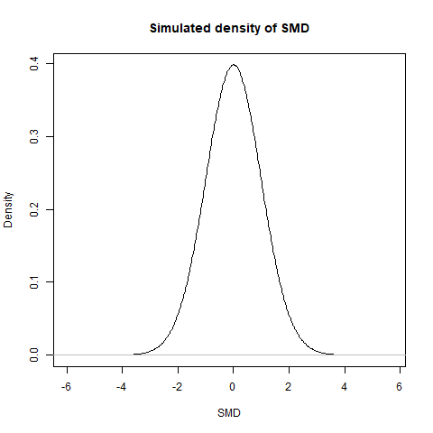
Simulating the distribution and its variance: Even with this approximation the distribution of the part inside the square-root is a convolution of gamma distributions that does not exist in closed form unless $n_1=n_2$ (in which case it is a gamma distribution). This means that the distribution of $T$ is easiest to find by simulation. It can be simulated to high accuracy by creating a kernel density for values simulated from this distribution:
#Create function to simulate kernel density of SMD using m generated values
SMD_DENSITY <- function(n1, n2, s1, s2, m = 10^7) {
    Z  <- rnorm(m,0,1);
    C1 <- rchisq(m, n1-1)/(n1-1);
    C2 <- rchisq(m, n2-1)/(n2-1);
    w  <- (s1^2/n1)/(s1^2/n1 + s2^2/n2);
    T  <- Z/sqrt(w*C1+(1-w)*C2);
    list(VALS = T, DENSITY = density(T));  }

#Example of simulated density
set.seed(12345);
n1 <- 50;
n2 <- 60;
s1 <- 6;
s2 <- 12;
TT <- SMD_DENSITY(n1, n2, s1, s2);
plot(TT$DENSITY, main = 'Simulated density of SMD',
         xlab = 'SMD', ylab = 'Density');

#Find variance of SMD
var(TT$VALS);
[1] 1.023165


