Autocorrelation in residuals

Question

Hi guys, thanks for your time!

Problem description:

I am working with dynamic factors. I have 4 panels of 24 series (hourly electricity prices) and I reduce them to 1 dynamic factor each that I then use as an index. The following discussion is based on the factors.

I am running an OLS model yt = b0 + b1x1t + b2x2t + b3x3t + et

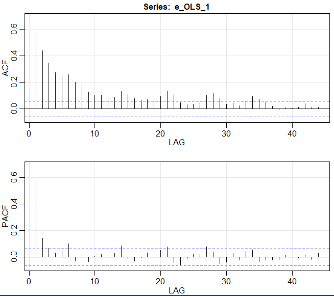
I can see that et is autocorrelated of order 4 (AR(4)).

I then use GLS with AR(4) but the residuals still appear the same as of the first OLS (the one with with no AR structure).

I use the nlme::gls in R

I also use orcutt::cochrane.orcutt, same story.. 100% same residuals as from the original OLS.

Could it be I am doing something wrong?

You can see some of my R code bellow:

Cochrane.orcutt

m1_adj <- orcutt::cochrane.orcutt(m1)

summary(m1_adj)

acf2(m1_adj$residuals)

GLS errors

m2 <- gls(y~ x1 + x2 + x3, correlation = corARMA(form = ~ 1,p=4,q=0))

summary(m2)

ef <- m2$residuals

acf2(ef)

I also run the Cochrane.orcutt in GRETL and there it seems to somewhat fix the autocorrelation problem with AR(1) residuals.

However, I cannot really find a model that perfectly solves the autocorrelation issue in my residuals. I also tried ARFIMA models and they also cannot fix it fully. I tried seasonal models as well.

Any suggestions are welcome of how to deal with my autocorrelation in the residuals!

Plots

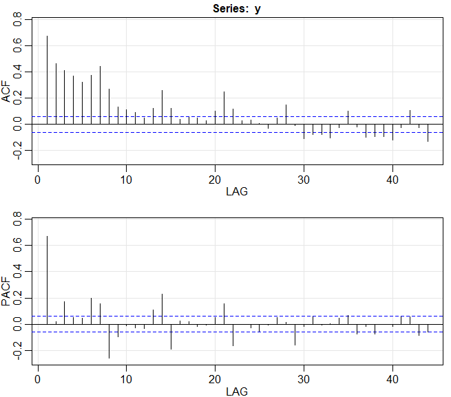
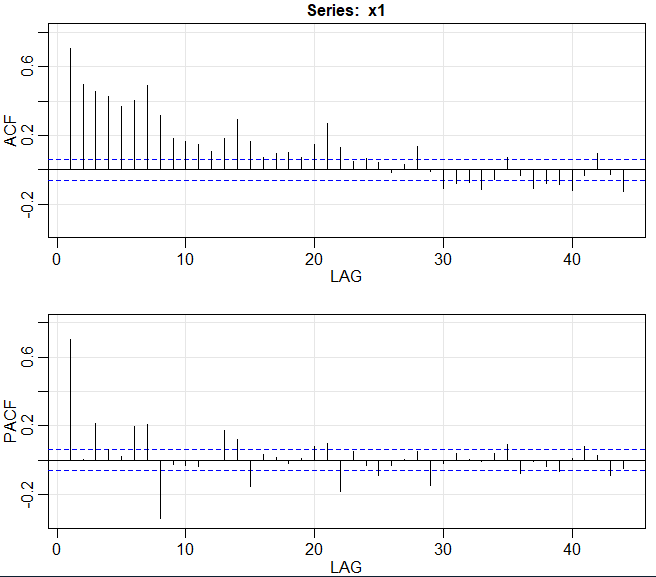
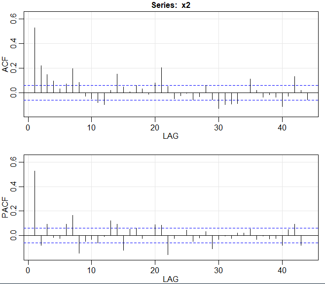
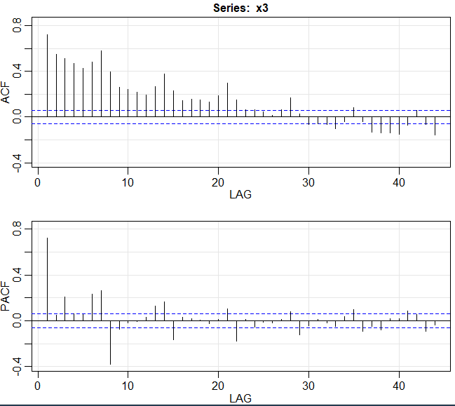
You can see plots of my variables bellow:

please note that what appears as weekly seasonality is not deterministic so including weekly dummies or using SARIMA with weekly seasonality doesn't change a thing. I think it comes from fractional integration but the AFRIMA doesn't really solve the issue..

Answer 1

I have now figured out the weird behavior.

My series have long-memory and the factors that I estimate are very sensible to non-stationarity which has moved as an non-deterministic effect to the final variables.

However, after estimating the long-memory dependencies and differencing with the fractional parameter estimated with Local Whittle techniques my factors were no longer non-stationary and all the weird behavior disappeared.

I was able to estimate the relationship between the factors perfectly.