Why use a Gaussian mixture model?

Question

I am learning about Gaussian mixture models (GMM) but I am confused as to why anyone should ever use this algorithm.

1. How is this algorithm better than other standard clustering algorithm such as $K$-means when it comes to clustering? The $K$ means algorithm partitions data into $K$ clusters with clear set memberships, whereas the Gaussian mixture model does not produce clear set membership for each data point. What is the metric to say that one data point is closer to another with GMM?

2. How can I make use of the final probability distribution that GMM produces? Suppose I obtain my final probability distribution $f(x|w)$ where $w$ are the weights, so what? I have obtained a probability distribution that fits to my data $x$. What can I do with it?

3. To follow up with my previous point, for $K$ means, at the end we obtain a set of $K$ clusters, which we may denote as the set $\{S_1, \ldots, S_K\}$, which are $K$ things. But for GMM, all I obtain is one distribution $f(x|w) = \sum\limits_{i=1}^N w_i \mathcal{N}(x|\mu_i, \Sigma_i)$ which is $1$ thing. How can this ever be used for clustering things into $K$ cluster?

Answer 1

I'll borrow the notation from (1), which describes GMMs quite nicely in my opinon. Suppose we have a feature $X \in \mathbb{R}^d$. To model the distribution of $X$ we can fit a GMM of the form

$$f(x)=\sum_{m=1}^{M} \alpha_m \phi(x;\mu_m;\Sigma_m)$$ with $M$ the number of components in the mixture, $\alpha_m$ the mixture weight of the $m$-th component and $\phi(x;\mu_m;\Sigma_m)$ being the Gaussian density function with mean $\mu_m$ and covariance matrix $\Sigma_m$. Using the EM algorithm (its connection to K-Means is explained in this answer) we can aquire estimates of the model parameters, which I'll denote with a hat here ($\hat{\alpha}_m, \hat{\mu}_m,\hat{\Sigma}_m)$. So, our GMM has now been fitted to $X$, let's use it!

This addresses your questions 1 and 3

What is the metric to say that one data point is closer to another with GMM?
[...]
How can this ever be used for clustering things into K cluster?

As we now have a probabilistic model of the distribution, we can among other things calculate the posterior probability of a given instance $x_i$ belonging to component $m$, which is sometimes referred to as the 'responsibility' of component $m$ for (producing) $x_i$ (2) , denoted as $\hat{r}_{im}$

$$ \hat{r}_{im} = \frac{\hat{\alpha}_m \phi(x_i;\mu_m;\Sigma_m)}{\sum_{k=1}^{M}\hat{\alpha}_k \phi(x_i;\mu_k;\Sigma_k)}$$

this gives us the probabilities of $x_i$ belonging to the different components. That is precisely how a GMM can be used to cluster your data.

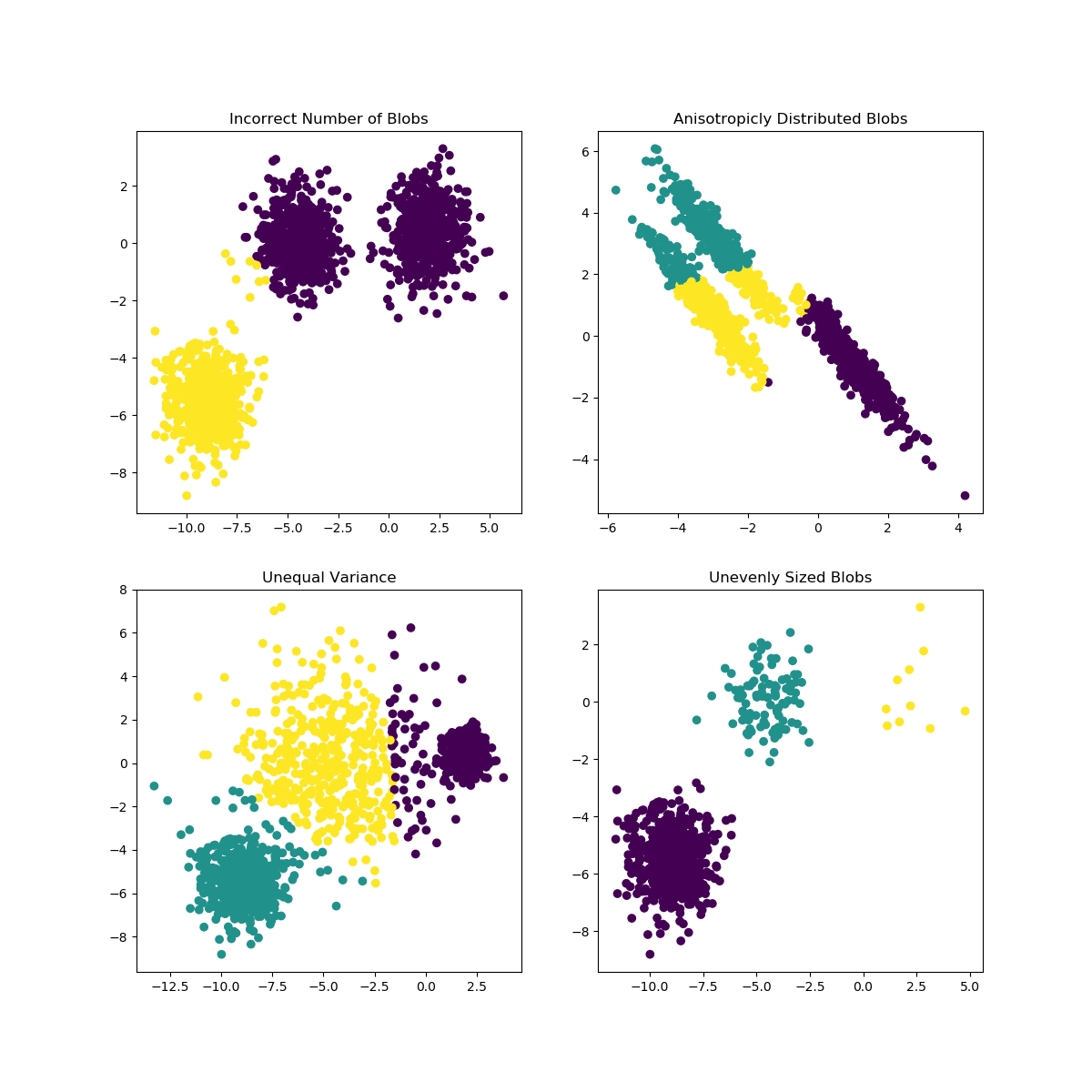
K-Means can encounter problems when the choice of K is not well suited for the data or the shapes of the subpopulations differ. The scikit-learn documentation contains an interesting illustration of such cases

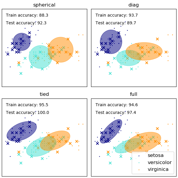
The choice of the shape of the GMM's covariance matrices affects what shapes the components can take on, here again the scikit-learn documentation provides an illustration

While a poorly chosen number of clusters/components can also affect an EM-fitted GMM, a GMM fitted in a bayesian fashion can be somewhat resilient against the effects of this, allowing the mixture weights of some components to be (close to) zero. More on this can be found here.

References

(1) Friedman, Jerome, Trevor Hastie, and Robert Tibshirani. The elements of statistical learning. Vol. 1. No. 10. New York: Springer series in statistics, 2001.
(2) Bishop, Christopher M. Pattern recognition and machine learning. springer, 2006.

Answer 2

1. How is this algorithm better than other standard clustering algorithm such as $K$-means when it comes to clustering?

• k-means is well suited for roughly spherical clusters of equal size. It may fail if these conditions are violated (although it may still work if the clusters are very widely separated). GMMs can fit clusters with a greater variety of shapes and sizes. But, neither algorithm is well suited for data with curved/non-convex clusters.

• GMMs give a probabilistic assignment of points to clusters. This lets us quantify uncertainty. For example, if a point is near the 'border' between two clusters, it's often better to know that it has near equal membership probabilities for these clusters, rather than blindly assigning it to the nearest one.

• The probabilistic formulation of GMMs lets us incorporate prior knowledge, using Bayesian methods. For example, we might already know something about the shapes or locations of the clusters, or how many points they contain.

• The probabilistic formulation gives a way to handle missing data (e.g. using the expectation maximization algorithm typically used to fit GMMs). We can still cluster a data point, even if we haven't observed its value along some dimensions. And, we can infer what those missing values might have been.

1. ...The $K$ means algorithm partitions data into $K$ clusters with clear set memberships, whereas the Gaussian mixture model does not produce clear set membership for each data point. What is the metric to say that one data point is closer to another with GMM?

GMMs give a probability that each each point belongs to each cluster (see below). These probabilities can be converted into 'hard assignments' using a decision rule. For example, the simplest choice is to assign each point to the most likely cluster (i.e. the one with highest membership probability).

2. How can I make use of the final probability distribution that GMM produces? Suppose I obtain my final probability distribution $f(x|w)$ where $w$ are the weights, so what? I have obtained a probability distribution that fits to my data $x$. What can I do with it?

Here are just a few possibilities. You can:

• Perform clustering (including hard assignments, as above).

• Impute missing values (as above).

• Detect anomalies (i.e. points with low probability density).

• Learn something about the structure of the data.

• Sample from the model to generate new, synthetic data points.

3. To follow up with my previous point, for $K$ means, at the end we obtain a set of $K$ clusters, which we may denote as the set $\{S_1, \ldots, S_K\}$, which are $K$ things. But for GMM, all I obtain is one distribution $f(x|w) = \sum\limits_{i=1}^N w_i \mathcal{N}(x|\mu_i, \Sigma_i)$ which is $1$ thing. How can this ever be used for clustering things into $K$ cluster?

The expression you wrote is the distribution for the observed data. However, a GMM can be thought of as a latent variable model. Each data point is associated with a latent variable that indicates which cluster it belongs to. When fitting a GMM, we learn a distribution over these latent variables. This gives a probability that each data point is a member of each cluster.