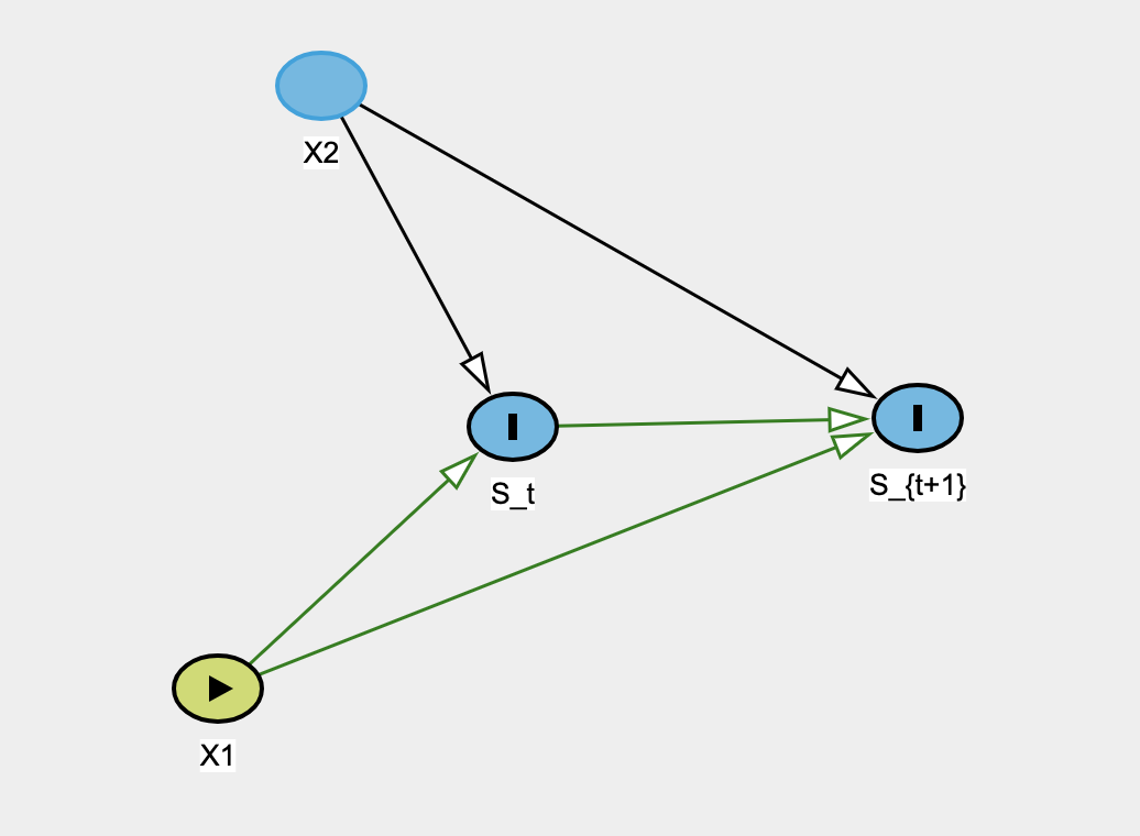
For linear regression, if $y$ actually depends on two positively correlated covariates $x_1$ and $x_2$ (we can call it the true model), and if we only include one covariate, say $x_1$, in the regression model (we can call it the working model), its coefficient $\beta_1$ will be overestimated. This makes intuitive sense, because now $\beta_1$ represents the effect of both $x_1$ and $x_2$. One can in fact derive that $\tilde{\beta}_1 = \beta_1 + \rho \beta_2$, where $\tilde{\beta}_1$ is the apparent coefficient of $x_1$ in the working model, $\beta_1$ and $\beta_2$ are the actual coefficients of $x_1$ and $x_2$ in the true model, and $\rho$ is the correlation coefficient between $x_1$ and $x_2$. (The derivation is appended at the end.)
Now I am interested in the same question for Cox proportional hazard model. To my surprise, I observe that when the true model has positively-correlated $x_1$ and $x_2$, and the working model has only $x_1$, $\beta_1$ is in fact underestimated, at least when estimated using Cox's partial likelihood method. Here are my simulation codes with some explanatory comments.
library(mvtnorm)
library(survival)

n <- 100000
set.seed(0)

# set the correlation coefficient to be 0.5
sigma <- matrix(c(1,0.5,0.5,1), ncol=2)
X <- rmvnorm(n=n, mean=c(0,0), sigma=sigma)

x1 <- X[,1]
x2 <- X[,2]

b1 <- 1
b2 <- 3

# relative hazards
relhazs <- exp(b1*x1 + b2*x2)

# event times
# assume baseline hazard is a constant function at 1
# so the survival times are simply exp distributed
etimes <- rexp(n, relhazs)

# assume no censorship for simplicity
status <- rep(1, n)

dat <- data.frame(id=1:n,
                  time=etimes,
                  status=status,
                  x1=x1,
                  x2=x2)
Output:
Call:
coxph(formula = Surv(time, status) ~ x1 + x2, data = dat, control = coxph.control(timefix = FALSE))

        coef exp(coef)  se(coef)     z      p
x1  1.004289  2.729965  0.004424 227.0 <2e-16
x2  2.991976 19.925012  0.008271 361.7 <2e-16

Likelihood ratio test=236231  on 2 df, p=< 2.2e-16
n= 100000, number of events= 1e+05
Call:
coxph(formula = Surv(time, status) ~ x1, data = dat, control = coxph.control(timefix = FALSE))

       coef exp(coef) se(coef)     z      p
x1 0.837905  2.311519 0.003825 219.1 <2e-16

Likelihood ratio test=49198  on 1 df, p=< 2.2e-16
n= 100000, number of events= 1e+05
My questions:
- Why the underestimation?
- Can we possibly derive some analytical relationship between $\tilde{\beta}_1$, $\beta_1$, $\beta_2$ and $\rho$ in this case, just like what we did for linear regression, even for some simple baseline distribution such as $\text{Exp}(1)$ in my simulation?
- If I estimate the parameters using a parametric model, then $\beta_1$ is indeed overestimated (please see below). Why the difference between Cox's semi-parametric partial-likelihood-based estimation and parametric full-likelihood-based estimation?
Call:
survreg(formula = Surv(time, status) ~ x1 + x2 + 0, data = dat,
    dist = "exp")

Coefficients:
       x1        x2
-1.004653 -2.993058

Scale fixed at 1

Loglik(model)= -100274.9   Loglik(intercept only)= -655669.9
    Chisq= 1110790 on 1 degrees of freedom, p= <2e-16
n= 100000
Call:
survreg(formula = Surv(time, status) ~ x1 + 0, data = dat, dist = "exp")

Coefficients:
      x1
-2.50526

Scale fixed at 1

Loglik(model)= -1302576   Loglik(intercept only)= -655669.9
n= 100000
Appendix:
For linear regression, suppose the true model is $y=\beta_1 x_1 + \beta_2 x_2 + \epsilon$, and the working model is $y=\tilde{\beta}_1 x_1 + \tilde{\epsilon}$. Without the loss of generality, assume $x_1$ and $x_2$ are standardized, so $x_2=\rho x_1$ where $\rho$ is the correlation coefficient. Equating the $y$ in the two equations and plugging in $x_2=\rho x_1$ give $\tilde{\beta}_1 = \beta_1 + \rho \beta_2$.


survregis actually not estimating the proportional hazards, but an AFT model. To illustrate side by side, seelibrary(icenReg); fit_ph = ic_par(cbind(time, time) ~ x1, data = dat, model = "ph");fit_ph; fit_aft = ic_par(cbind(time, time) ~ x1, data = dat, model = "aft");fit_aftat the end of your code. Note that settingmodel = "ph"gives nearly identical coefficients ascoxph! $\endgroup$x2being absorbed into the baseline distribution, you no longer have an exponential distribution, meaning you no longer have constant hazards and no longer have proportional hazards inx1. However, your simulation properly sits inside an AFT model (although you've miss specified the baseline distribution, of course). $\endgroup$