The definition of a confounder is somewhat complicated, but VanderWeele & Shpitser (2013) decided
A pre-exposure covariate C is a confounder for the effect of A on Y if
it is a member of some minimally sufficient adjustment set.
A sufficient adjustment set is a set of variables conditioning on which is sufficient to remove confounding. Using the language of causal graphs, it is a set of variables that blocks all back-door paths from treatment to the outcome and doesn't block any front-door paths. A minimally sufficient adjustment set is a sufficient adjustment set for which no proper subset is also a sufficient adjustment set.
The main result of Rosenbaum & Rubin (1983) is that, for a sufficient adjustment set, it is sufficient to condition on the conditional probability of treatment given that same set of variables to eliminate confounding. Formally, consider the collection $X$ of all variables $x_1, ... x_k$ that are not caused by the treatment ($A$) or outcome ($Y$). Now consider a subset of $X$, called $V$. If $Y^A \perp A|V$, that is, if $V$ is a sufficient adjustment set, then $Y^A \perp A|e(V)$, where $e(V)=P(A=1|V)$ is the propensity score. This means that we can estimate a treatment effect within strata of $e(V)$, and those treatment effects will be unbiased (i.e., free of confounding). This is what justifies propensity score matching, subclassification, and regression (although these all have additional requirements and assumptions, so don't go running off using them without understanding what else is required and how these techniques differ).
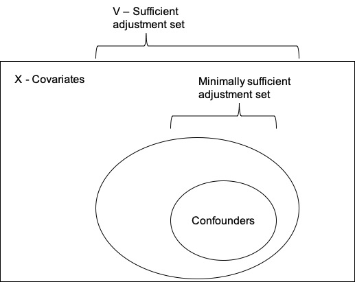
"Covariate" is usually not rigorously defined in the context of causal inference. It usually refers to $X$, the collection of variables not caused by treatment, some of which form a sufficient adjustment set. $X$ usually contains confounders, instrumental variables (variables that cause selection into treatment but have no direct effect on the outcome), prognostic variables (variables that cause variation in the outcome but are independent of the treatment), and irrelevant variables (variables that cause neither selection into treatment nor variation in the outcome). There may also be some bias-inducing variables that, when conditioned upon, induce bias in an effect estimate.
In propensity score (and other causal) analyses, it is up to the researcher to select a subset of $X$, namely $V$, that is a sufficient adjustment set. $V$ will then contain confounders (i.e., variables part of a minimally sufficient adjustment set) and other covariates (if any). Typically theory is used to select $V$, though there have been some attempts to use machine learning to select them (e.g., Shortreed & Ertefaie, 2017; Koch, Vock, & Wilson, 2018).
To sum up, a treatment effect estimate is unbiased conditional on a sufficient adjustment set. It is also unbiased conditional on a propensity score formed from that sufficient adjustment set. A sufficient adjustment set is a subset of variables not caused by treatment, often called covariates, that is sufficient to remove confounding. A confounder is a member of a minimally sufficient adjustment set. Adjustment sets will contain confounders and, though not necessarily, other covariates. Here's a Venn diagram to display these distinctions:

Koch, B., Vock, D. M., & Wolfson, J. (2018). Covariate selection with group lasso and doubly robust estimation of causal effects. Biometrics, 74(1), 8–17.
Rosenbaum, P. R., & Rubin, D. B. (1983). The central role of the propensity score in observational studies for causal effects. Biometrika, 70(1), 41–55.
VanderWeele, T. J., & Shpitser, I. (2013). On the definition of a confounder. Annals of Statistics, 41(1), 196–220.
Shortreed, S. M., & Ertefaie, A. (2017). Outcome-adaptive lasso: Variable selection for causal inference: Outcome-Adaptive Lasso. Biometrics, 73(4), 1111–1122.

