R result interpretation conditional inference tree result for nominal response

Question

I have nominal responses, "yes/no/don't know", that I am using in a conditional inference tree in R. I am having trouble with how to interpret the model's output concerning one of the independent variables: gender. There are other independent variables, like income or education, but the model picks gender as first split even among all independent variables.

A small bit of the data. There are 2328 rows, so I only provided a small number to give an idea of the data:

library(partykit)
dput(head(know_nt))
structure(list(know_nt = structure(c(3L, 3L, 3L, 3L, 3L, 3L), .Label = c("No", 
"Don't know", "Yes"), class = "factor"), gender = structure(c(1L, 
1L, 2L, 1L, 1L, 1L), .Label = c("female", "male"), class = "factor")), row.names = c(1L, 
2L, 3L, 4L, 6L, 7L), class = "data.frame")

know_nt %>% group_by(know_nt, gender) %>% summarize(n())
# A tibble: 6 x 3
# Groups:   know_nt [3]
know_nt    gender `n()`
<fct>      <fct>  <int>
1 No         female    37
2 No         male      12
3 Don't know female    73
4 Don't know male      24
5 Yes        female  1261
6 Yes        male     921

My model is

ctree(know_nt ~ gender, data= know_nt)

Model formula:
know_nt ~ gender

Fitted party:
[1] root
|   [2] gender in female: Yes (n = 1371, err = 8.0%)
|   [3] gender in male: Yes (n = 957, err = 3.8%)

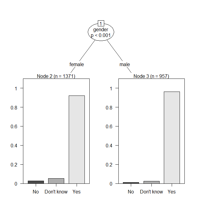
The plot looks like

I think I am misunderstanding the output. By looking at the plot, where there is a split on male and female, I thought that meant that one gender responded in one way to knowing about nt and the other gender responded in a different way. For example, the male responses selected yes and the female responses selected either no or don't know. But the print of the model says yes for both genders. How is that? How should this be interpreted? If yes is indicative for both genders, why is there a split?

Answer 1

The most common answer is yes on both branches, but there is a difference in the proportion of people choosing yes, no and don't know. So gender does have some predictive power, but it's likely quite small. As ReneBt says above, this is not a concern limited to decision trees - the difference between statistical significance and effect sizes is important to understand for a great deal of modelling approaches.

Answer 2

Just to add to the previous correct answers/comments of mkt and ReneBt: What ctree() does here is quite similar to a simple $\chi^2$ test in this two-way table. Thus, the tree doesn't add much you wouldn't get from a classical analysis.

First, I enter the data in tabulated form and then expand them to the raw format. The latter is not strictly necessary but is more convenient for some of the functions below.

d <- data.frame(
  know_nt = factor(c(1, 1, 2, 2, 3, 3), labels = c("No", "Don't know", "Yes")),
  gender = factor(c(1, 2, 1, 2, 1, 2), labels = c("female", "male")),
  n = c(37, 12, 73, 24, 1261, 921)
)
d <- d[rep(1:6, d$n), 1:2]

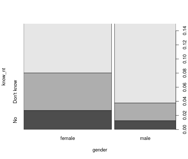
A very simple plot of this data is a flavor of stacked bar plot, known also as spine plot, which you can get from the basic plot() function:

plot(know_nt ~ gender, data = d, ylim = c(0, 0.15), tol.ylab = 0.01)

This shows that the No and Don't know categories combined are around 8% for females and less than 4% for males. Note that this exactly corresponds to the err = ... in the printed output from the tree in your question. Note also that the y-axis is limited at 15% so that most of the bar for the Yes category is not shown.

Although the differences in proportions are not very large, they are statistically significant due to the relatively large sample size. The classical $\chi^2$ test yields:

chisq.test(xtabs(~ gender + know_nt, data = d))
##  Pearson's Chi-squared test
## 
## data:  xtabs(~gender + know_nt, data = d)
## X-squared = 17.414, df = 2, p-value = 0.0001655

The conditional inference underlying this particular tree (with categorical response and categorical partitioning variable) also essentially runs a $\chi^2$ test. Thus, after fitting the tree with

tr <- ctree(know_nt ~ gender, data = d)

you can extract the test in the root node by

options(scipen = 10, digits = 4)
sctest.constparty(tr, node = 1)
##               gender
## statistic 17.4061167
## p.value    0.0001661

Up to some small differences in the standardization of the test statistic, this is the same test. And the predictions from the tree for the two nodes correspond exactly to what the spine plot above has visualized:

predict(tr, newdata = data.frame(gender = c("female", "male")), type = "prob")
##        No Don't know    Yes
## 1 0.02699    0.05325 0.9198
## 2 0.01254    0.02508 0.9624

In short, insights from classical techniques and the conditional inference tree are virtually identical. Whether or not the differences detected are relevant for you is a different matter, of course...