3
$\begingroup$

I programmed a feedforward neural network for forecasting a time series, but the forecast is not stable and reasonable. I used a non-seasonal lag of 3, hence produced a gliding window of 3 as input for the NN, meaning 3 y-values of the series were given as input and the next one was labeled for training. The forecasting then was done in an autoregressive manner. My method was similar to making a AR(3) model without noise and drift. I am not sure the network results are better than a random walk though.

Specification of the network: 2 hidden layers; First layer with 12 units and relu activation. Second one with 8 units and also relu. Output was of course linear and one dimensional. As loss the MSE was used and the loss was optimized with ADAM. Epochs = 400, batch size = 2. The input data was MinMax scaled between $[0,1]$.The whole data has 202 samples.

The validation set was created by using validation_split=0.15 from keras, which splits the last 15% of the training as test set. Both training and test were not shuffled to avoid temporal leaks.

I used R2 and MSE for goodness of fit. R2 training: 0.769, MSE training: 0.009, R2 test: 0.436, MSE test: 0.012

I tried different network topologies, optimizers and epochs. What surprises me is that this worked fine when using the nnetar function in R. This function only has one hidden layer and when configuring the same number of lags it produces very good results. It uses the BFGS algorithm and as far as I could read the source code does not involve regularization (The function also averages over different trained networks, but I still get results when I don't average).

The code and data I worked with will be provided soon. (Not sure yet in which form to provide it here, since the code is about 100 lines).

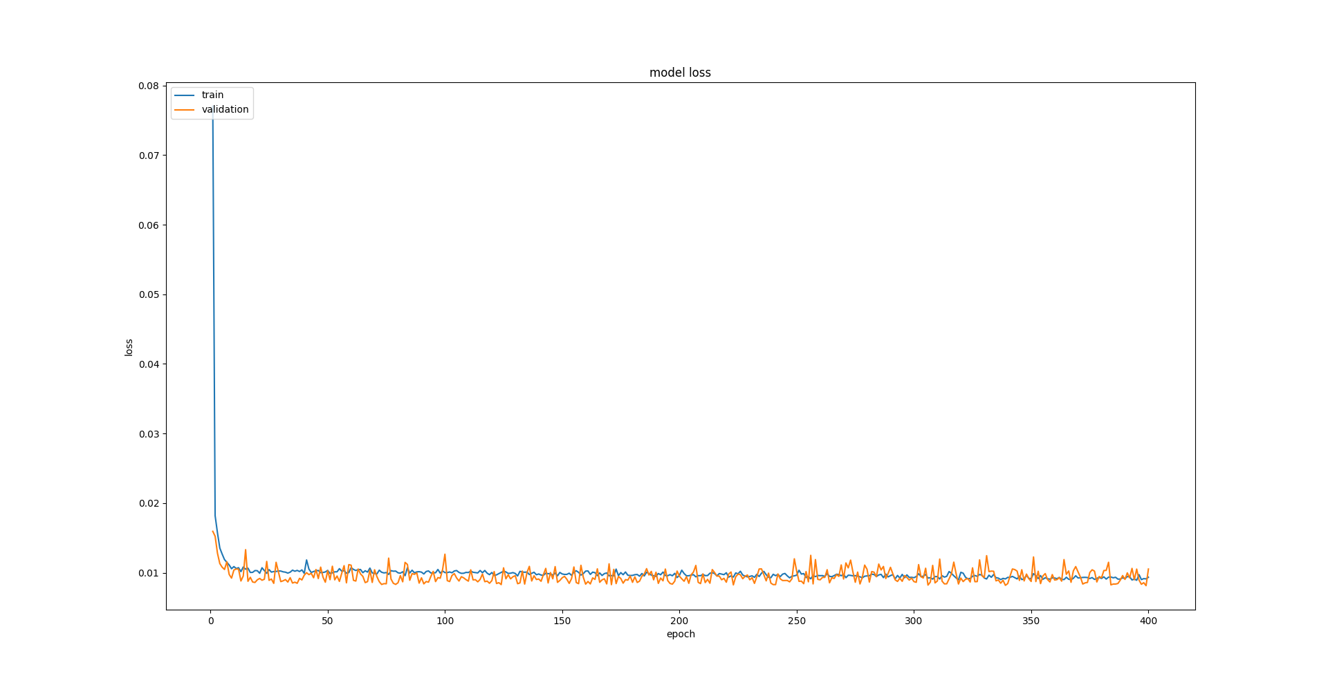
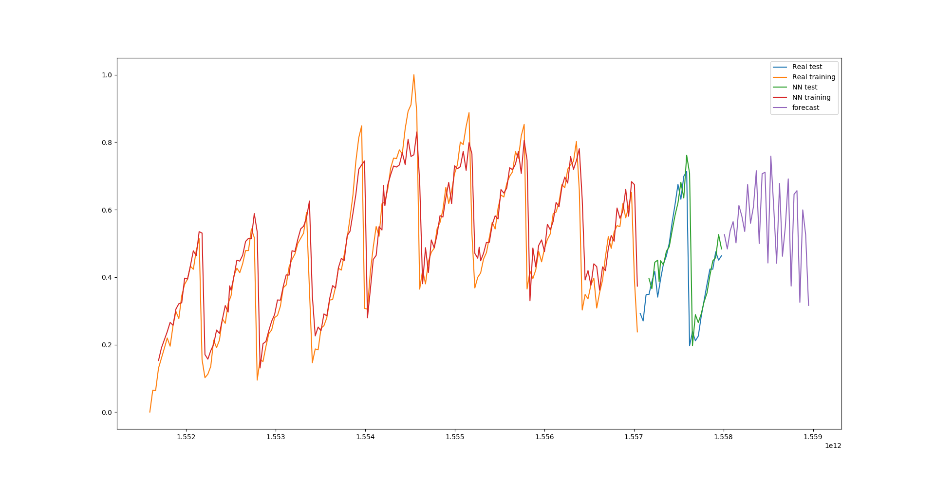
validation and train loss forecast plot

For the color labels of the time series plot:

  • Orange: The set used for training the NN
  • Red: NN output for the training data after being trained
  • Blue: The test data (NN has never seen this when being trained)
  • Green: NN output for the test data after being trained.
  • Voilet: The autoregressive forecast of the NN starting with the 3 last values of the test set for the first prediction. Then continue using the gliding window as explained
$\endgroup$
4
  • $\begingroup$ Post your data in a csv format . also precisely define what your colors represent . $\endgroup$
    – IrishStat
    Commented May 29, 2019 at 8:24
  • 1
    $\begingroup$ @IrishStat How can I post the csv? $\endgroup$ Commented May 29, 2019 at 8:30
  • $\begingroup$ that's a good question . I can't figure that out for myself .. I guess I am to old ...email it to me at my internet address and perhaps someone smarter than I can help us both how to attach an external file. One option is to use DROPBOX but that has some side effects. $\endgroup$
    – IrishStat
    Commented May 29, 2019 at 8:38
  • $\begingroup$ You may want to try a simpler model first to see what possible phenomena may be going on. Stationarity tests and autocorrelation may also provide information $\endgroup$
    – David
    Commented May 29, 2019 at 8:46

2 Answers 2

2
$\begingroup$

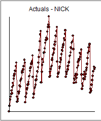
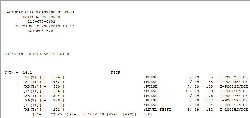
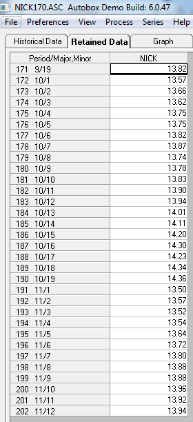
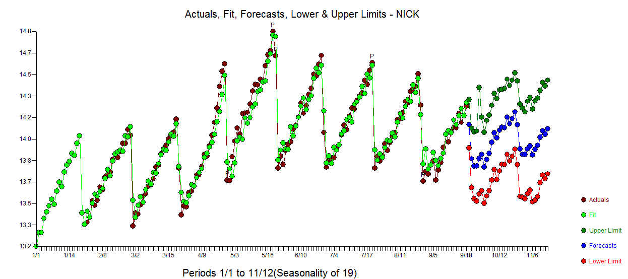
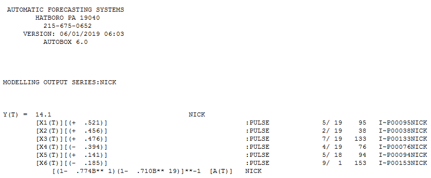
I am not an expert in NN but was intrigued by your question.I took your 202 sequential values enter image description here with known periodicity of 19 into AUTOBOX my tool of choice and proceeded to automatically analyze the data. It yielded the following model enter image description here suggesting a level shift at time period 152 in addition to a few pulses.

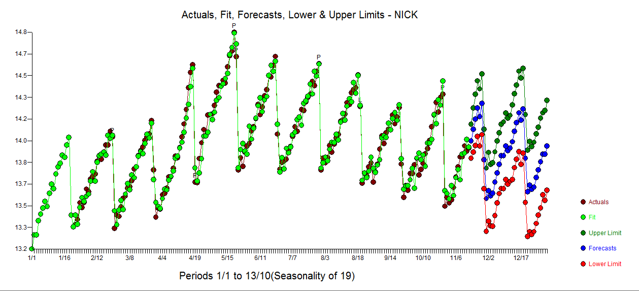
The Actual/Fit and Forecast graph as here enter image description here

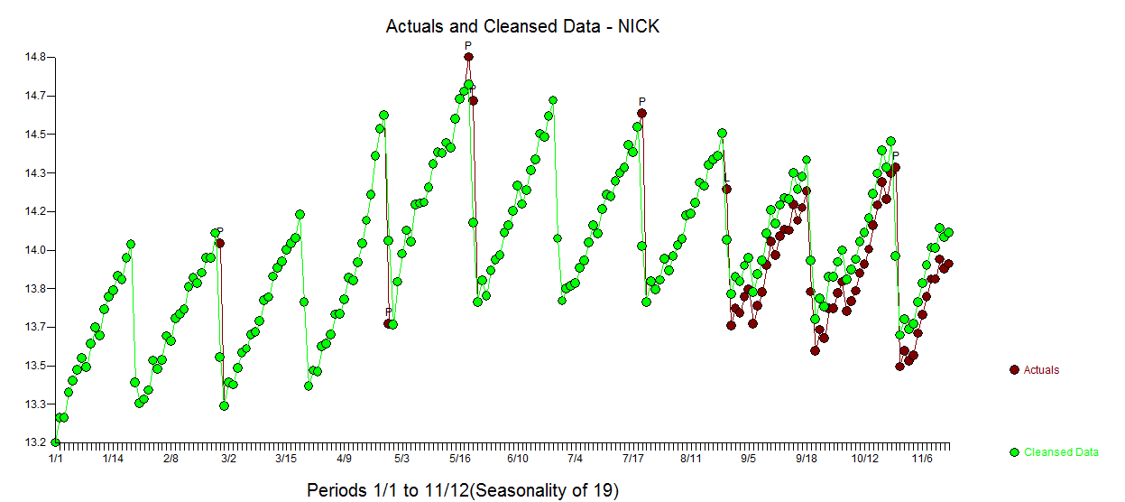
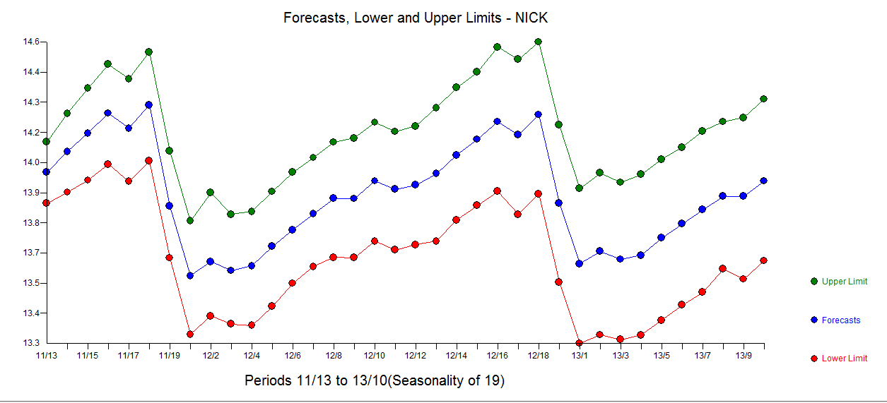
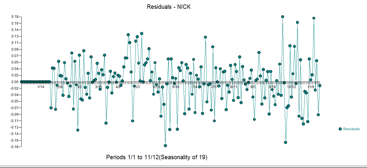
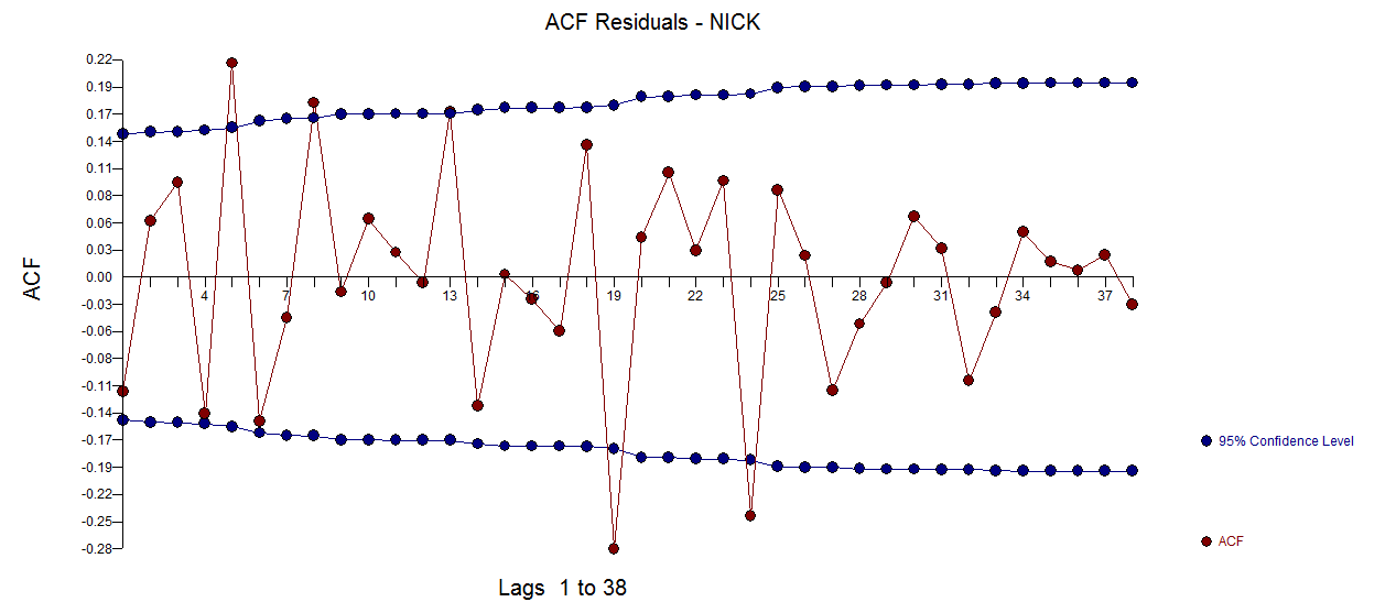
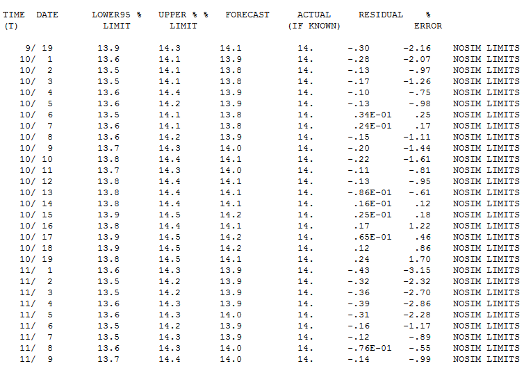
with cleansed data here enter image description here and reasonable forecasts here enter image description here . The plot of the model's residuals are here enter image description here with acf here enter image description here

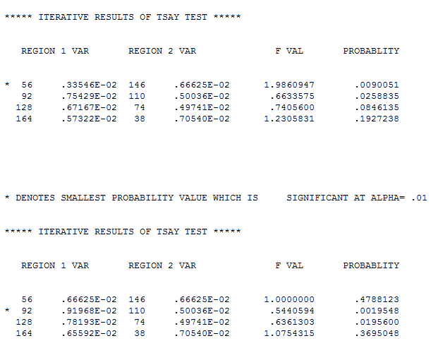
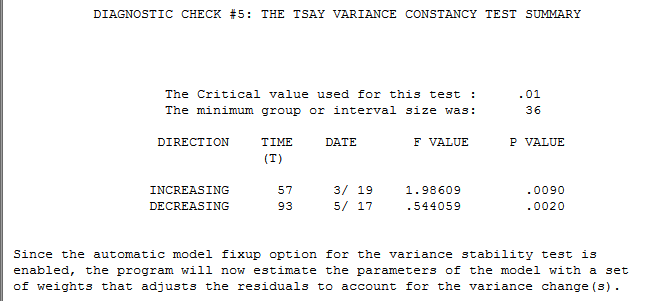
Note also that two change points were detected in the error varenter image description hereiance suggesting increased error variance at 56 and a reduction in error variance at 92 suggesting the need for Weighted Estimation (GLS) to render the error process homogeneous enter image description here

This all suggests to me that your simulation incorporated a deterministic (and ignored) component which might explain why your forecast is flawed as you only included stochastic memory (arima) while the data included additional deterministic effects and some error variance changes.

Do you concur with this ? Do you have any reason why your simulation may have introduced these additional effects NOT remediable with NN bit clearly in the historical .

To continue my research in this NN vs Robust Time Series I used your suggestion of 15% and retained 32 values from the end and proceeded to develop the following model and forecasts for the out-of-sample 32 values.

This is what was obtained using 172 actuals and 32 retained.

enter image description here and enter image description here and enter image description here .. no level shift at 152 due to only 20 values being available.

enter image description here and enter image description here with a 1.2% MAPE for the 32 periods.

I hope this helps you and others to clear up mysteries regarding NN and the possible analyses that are routinely available .

$\endgroup$
1
$\begingroup$

Based on the graph you posted, I would say you are falling into the "my fancy neural network is really just a random walk with drift" trap. If you look closely, you will notice that your forecasts are shifted by one step from the actuals: Your neural network just learned to copy the last value it saw and use it as the most likely next value $\pm$ a noise component (which is why it isn't an exact copy of the last value).

I don't have an exact answer, but here are two considerations:

  • You said you had better results with NNETAR with only one hidden layer? So why are you using 2 hidden layers then? That will only lead to overfitting. Unless you are modeling a really complex and/or multivariate time series, I do not recommend using multiple hidden layers for a forecasting problem.

  • Try training on multiple steps ahead instead of one step ahead, in my experience that led to better results and generally avoided the "random walk trap" which is so common when dealing with neural networks for forecasting.

$\endgroup$
1
  • $\begingroup$ Your answer is also very helpful! When using a single hidden layer, the forcast started showing structure after I implemented a seasonal lag of seasonality 16. (The TS actually has seasonality of 19, which is very strange to me, because with 19 it did not work). I am going to try multiple step forecasting, but for now I my focus is on just "copying" the output of NNETAR. Can you think of anything else that could be relevant? (Optimizer, epochs, regularizer,...) I might start a new thread with my latest results. $\endgroup$ Commented Jun 1, 2019 at 21:49

Your Answer

By clicking “Post Your Answer”, you agree to our terms of service and acknowledge you have read our privacy policy.

Not the answer you're looking for? Browse other questions tagged or ask your own question.